
1. Introduction
2. Procedure
3. Simple regression with SPSS
4. SPSS commands
5. Literature
Introduction
A simple linear regression analysis can be used for measuring the effect that one attribute has on another and for predicting one attribute by means of another. However, this is possible only if both variables are interval scaled and normal distributed. A simple linear regression analysis should always be chosen over a bivariate correlation analysis when drawing conclusions about the assumed direction of the correlation. In contrast to a multiple regression analysis with several independent variables, a simple linear regression analysis examines the influence an independent variable has on the dependent variable.
Problem definition
The direction of the relationship is straightforward in many questions. For example, it can be assumed that the number of umbrellas sold depends on the weather and not the other way around. In the case of other questions, however, the direction of the relationship is less obvious. But it is impossible to establish causality by means of a regression. It is therefore important to provide a strong theoretical basis for the assumed direction of the correlation. With the help of a regression analysis, it becomes possible to study the following types of questions:
- The cause analysis examines the size of the effect of the independent variable on the dependent variable.
- The impact analysis can be used for studying how the dependent variable reacts to a change in the independent variable.
- The prognosis allows for forecasts of the dependent variable concerning new values of the independent variable.
A simple regression analysis is therefore suitable for hypotheses such as “Does a person’s efficiency change when he or she is exposed to a lot of noise pollution at work?”, “If noise pollution at work increases by X, the person’s efficiency will change by Y.”, and “How does a person’s efficiency change when he or she is exposed to a lot of noise pollution at work?”.
Note: The term “regressand” is often used for the dependent variable, and “regressor” is often used for the independent variable
2. Procedure
How to conduct a regression analysis can now be explained based on the following question taken from the field of marketing research.
Do ad expenditures for a particular product influence the number of units sold?
A linear relationship between ad expenditures in CHF and the number of products sold can be assumed. It therefore follows that the number of units sold will increase if ad expenditures increase. The goal is to find out how strongly ad expenditures impact the sales figures of the product.
2.1 Hypothesis formulation
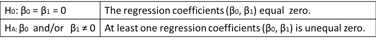
In order to test the research question statistically, it is necessary to formulate hypotheses. This means first coming up with hypotheses for reviewing the model as a whole, and then formulating hypotheses for reviewing the various regression coefficients. It should thus be possible to determine if the regression equation of the sample can be generalized onto the population.
1. The null hypothesis and the alternative hypothesis for the whole model are as follows:
Whereby the equation of the simple linear regression is formulated as:
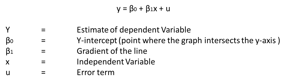
Note: The regression line is the line that minimizes the sum of the squared prediction errors (error term). There is always only one such line.
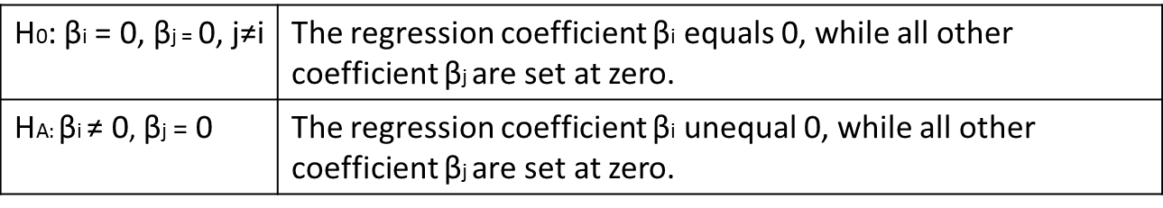
2. The null hypothesis and the alternative hypothesis for the various regression coefficients are as follows:
To test the hypothesis, it is first necessary to obtain data (see Table 1: Example file).
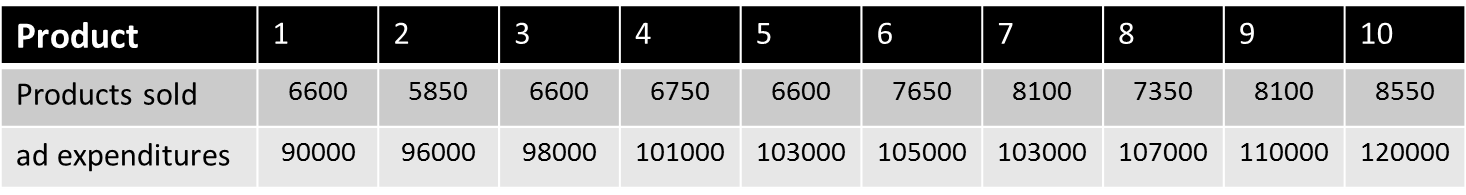
Table 1: Example file
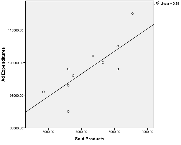
Figure 1: Scatter plot
The scatter plot indicates a linear correlation between the variables of “Ad expenditures” and “Number of products sold.”
2.2 Calculating the regression lines
The simple linear regression analysis aims to estimate the regression equation. In the case of a perfect linear correlation, all the points would fall onto a line. Figure 1: The scatter plot, however, shows that none of the data points are exactly on the line. These forecast errors, i.e. the difference between a particular observed value (data point) and the value as predicted by the regression line, are referred to as residuals. For this reason, it is necessary to calculate a line that minimizes the sum of the residuals. The Ordinary Least Squares Method (OLS) is generally used for this, which involves squaring and adding up the residuals of all data points and then minimizing the sum. The residuals are squared so that the larger distances can be weighted more strongly and the positive and negative distances don’t eliminate each other. This procedure produces the best estimated values of the coefficients of the population.
Quality of the regression model
The coefficient of determination R2 indicates how well the regression function fits with the empirical data. This is determined based on the residuals mentioned above. In general, R2 shows the part of the variance of the dependent variable that the regression function explains, whereby R2 as the standardized measure can take on values between 0 and 1.
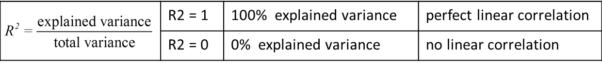
Note: When R2 takes on the maximum value of 1, the linear correlation is perfect, which means that all regression residuals equal zero.
The value of R2 increases with the number of independent variables regardless of whether other independent variables in fact contribute towards the explanatory power. The corrected coefficient of determination R2korr underscores this.
Note: In the case of a simple linear regression, the coefficient of determination R2 can also be calculated as the square of the correlation r between the observed and the estimated values of the dependent variable.
2.3 Conducting the hypothesis test
To predict an attribute in a sample meaningfully by means of a regression equation, it must be possible to generalize the attribute onto the population. Reviewing the regression function and the various regression coefficients for significance allows for such a generalization to be made.
- The F-test helps to verify if the estimated model is valid also for the population. Testing if a regression function can be generalized requires a comparison of the calculated F-test statistic with the theoretical value from the probability distribution. If the calculated F-value is greater than the critical F-value belonging to the previously determined significance level α, the null hypothesis that the regression coefficients (β0, β) as a group are equal to zero can be refused. The F-test thus makes it possible to draw a conclusion about the significance of the entire regression model.
- In addition to testing the regression model as a whole, the individual regression coefficients can also be tested for significance with the help of the t-statistic. Here, too, the calculated value is compared with the theoretical value of a probability function, in this case the one from the t-distribution. If the empirical value exceeds the critical value for the significance level α, the null hypothesis of the regression coefficient being equal to zero can be refused.
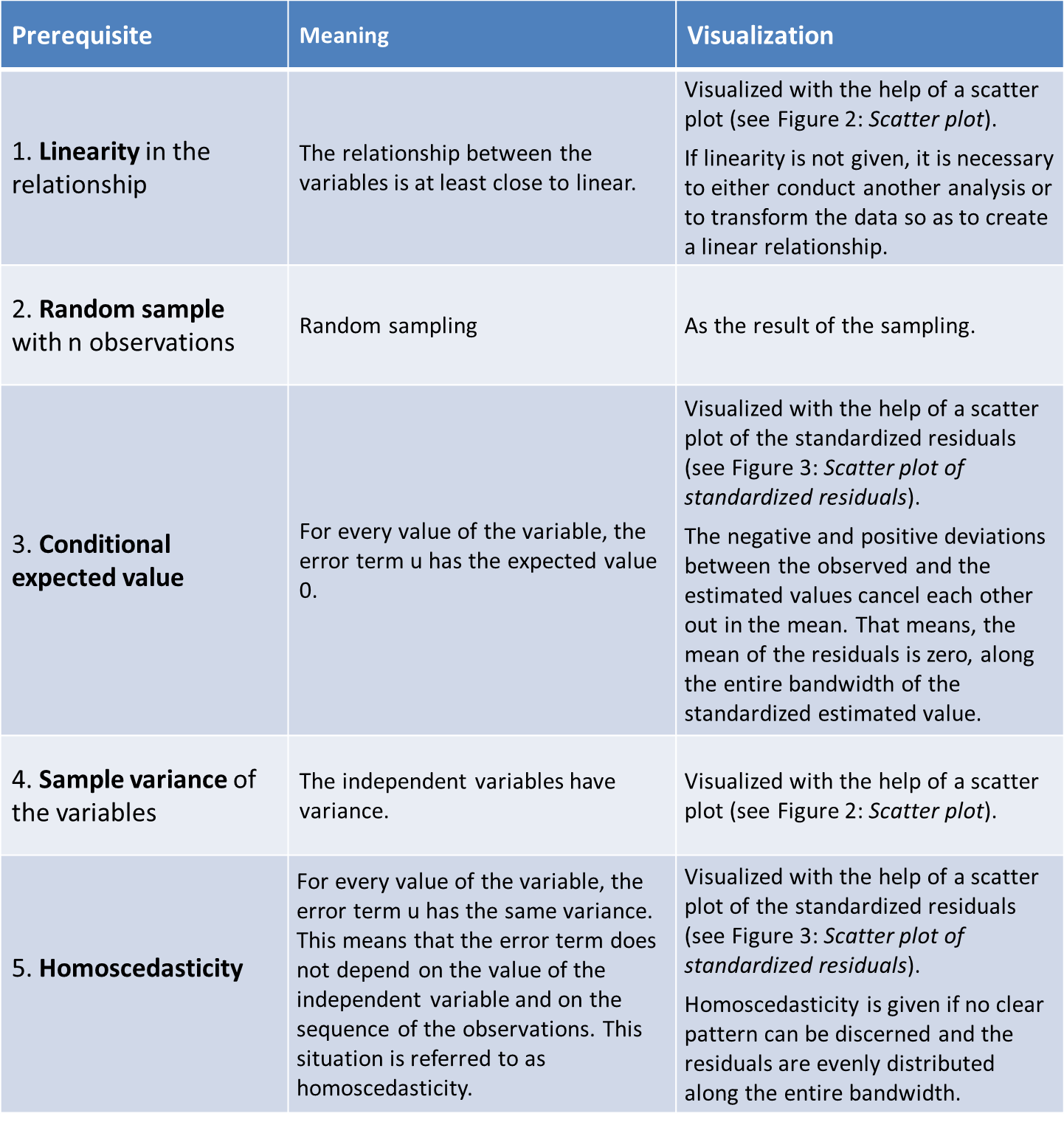
2.4 Testing the model’s prerequisites
Besides the prerequisite of normal distributed and interval scaled variables, the linear regression model is based on various assumptions. These are referred to as Gauss-Markov criteria, and they ensure that the OLS estimate of best, linear, unbiased estimator (BLUE) will generate the parameter (β0, β1) of the population.
These are the (see Wooldridge (2005))…
The linear regression model is based on two further assumptions. These are (see Wooldridge (2005))
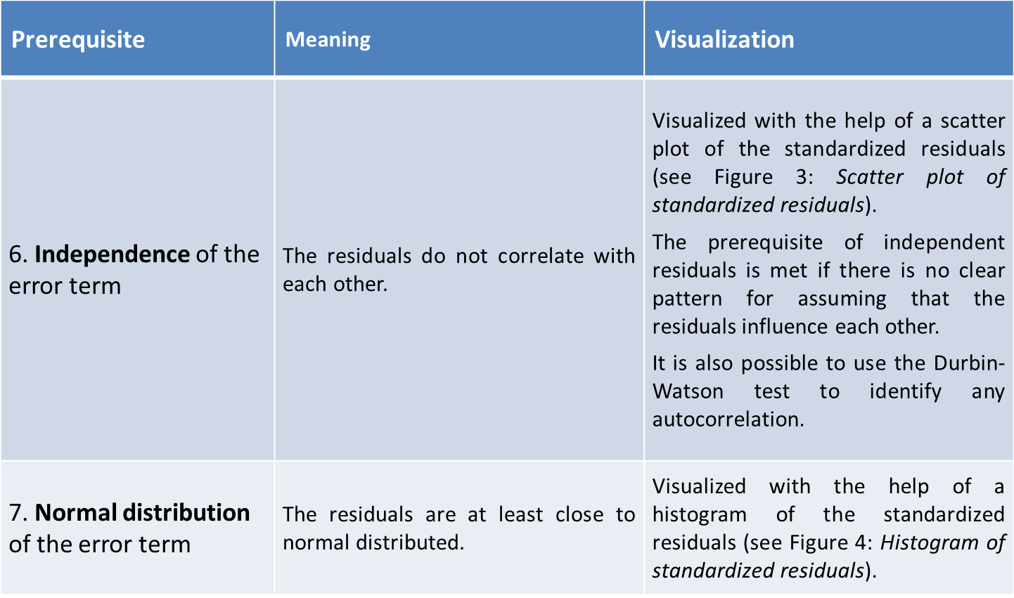
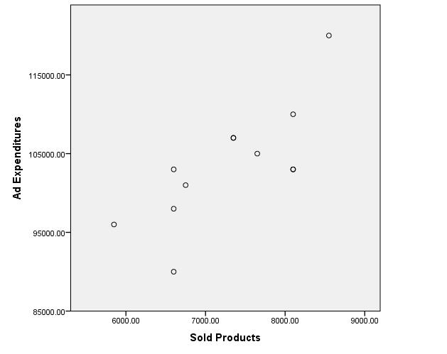
Figure 2: Scatter plot
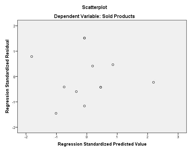
Figure 3: Scatter plot of standardized residuals
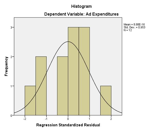
Figure 4: Histogram of standardized residuals
3. Simple regression with SPSS
The following figures show the results of the simple linear regression in the sequence as produced by SPSS.
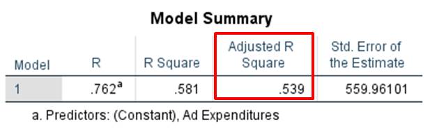
Figure 5: Coefficient of determination
The value of the corrected R2 equals .539 (see Figure 5: “Coefficient of determination”). This means that the regression model can explain 53.9% of the variance of the “Number of products sold” variable.
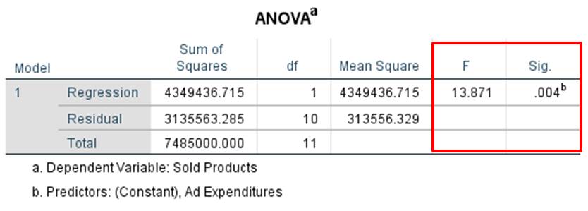
Figure 6: “Testing the regression function”
From the table in Figure 6: “Testing the regression function,” it is possible to obtain the F-value and the associated significance level (p-value). As a rule of thumb, the generated p-value must be less than .050. For this example, SPSS produces an F-statistic of 13.871 and a significance (p-value) of .004. Because the p-value is less than .050, it can be assumed that there is a statistical correlation between the “Ad expenditures” and “Number of products sold” variables.
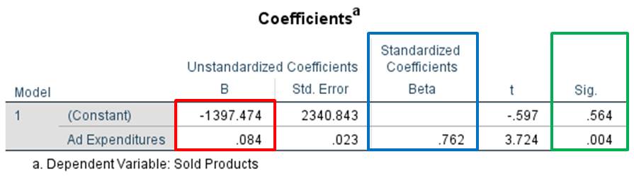
Figure 7: “Testing the regression coefficients”
From Figure 7: “Testing the regression coefficients” it is possible to obtain the regression coefficients of the regression lines and of the standardized regression equation. The upper value in the red column (labeled as “Constant”) refers to the section of the Y axis; the lower value (labeled as “ausgaben”) refers to the slope of the regression line. The column marked blue shows the standardized regression coefficients. Because the standardized line does not have a section of the Y axis, no value can be attributed to the constant in this case. The last column shows the significance level of the regression coefficients.
The regression coefficients from Figure 7: “Testing the regression coefficients” can help with calculating the regression coefficient in our example. The constant β0 in this model is not significant and does not create a problem in the case of a simple linear regression. A non-significant β0 value means that the regression line crosses the Y axis at point zero and thus passes through the origin. The non-standardized regression coefficient β for “Number of products sold” differs significantly from zero (p=.004) and has a value of .762. The estimated regression function in this case is:
y = .762x or “Number of products sold” = .762 × “Ad expenditures”
A CHF 1 increase in ad expenditures would thus result in 0.762 additional products sold.
Note: In this depiction of the regression lines it is important to pay attention to which units the variables have. It is therefore not possible to draw conclusions about the strength of the correlation based on the value of β. Furthermore, the regression coefficients of the various analyses cannot be compared with each other. SPSS produces the non-standardized regression coefficient as well as the standardized ones (see Figure 7: “Testing the regression coefficients”). In the case of a standardized equation, the value is the constant β0 = 0, which means the line passes through the origin. The standardized equation makes it possible to determine how strong the correlation is and if it is significant. The standardized equation is very important, especially in the case of a multiple regression analysis, because it is the only way of determining which independent variable has the strongest influence on the dependent variable. However, this equation does not allow for calculating an estimate of the dependent variables.
4. SPSS commands
Click sequence:
Regression: Analyze ► Regression ► Linear
Scatter plot: Diagrams ► Create diagram ► Simple scatter plot
(For the regression line in the SPSS output, double-click on the diagram and select “Adjustment line” for the overall value.)
Syntax:
Regression: REGRESSION
Histogram: /RESIDUALS HISTOGRAM(ZRESID)
Scatter plot of residuals: /SCATTERPLOT=(*ZRESID ,*ZPRED)