1. Introduction
2. Procedure
3. Multiple regression with SPSS
4. SPSS commands
5. Literature
1. Introduction
The multiple regression analysis is a widely used multivariate model, especially in empirical social research and market research. Unlike in the case of the simple linear regression analysis (LINK), multiple regressions allow for more than one independent variable to be included in a model. It can also be used to show and quantify causal relationships (analysis of causes) and predict the characteristic of the dependent variable (forecast).
For example, a multiple regression can be used to examine the following questions:
To what extent can several independent variables predict a dependent variable?
Do independent variables indicate an interaction effect or do they have a joint impact on a dependent variable that goes beyond the respective separate impacts?
What additional value for the prediction does a certain independent variable have if the effect of other independent variables on a dependent variable has already been considered?
2. Procedure
The procedure for conducting a regression analysis can be summarized in five steps, which are described in the following section.
2.1 Formulating the regression model
When formulating the regression model, practical and theoretical considerations play an important role, whereby assumptions are made about causes and effects. Before conducting a regression analysis, it is therefore necessary to decide which factor or factors to include as dependent variable(s) and which to include as independent variable(s) in the model. When calculating a multiple regression, the dependent variable must be at least interval scaled.
Mono-causal relationships are rarely found in empirical social research and market research, and a particular dependent variable is usually influenced by several independent variables (Figure 1). Therefore, a multiple regression is considered to be an extremely important statistical procedure.
Figure 1: The dependent variable is influenced by several factors
The following question serves as an example for calculating a multiple regression:
Which factors influence the average life expectancy in various countries?
The model that goes with this question could look as follows:
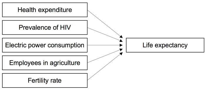
Figure 2: Example model
2.2 Estimating the regression function
This section explains how to estimate a particular regression function based on empirical data. Table 1 shows the six mentioned variables of 70 countries from the year 2008, data that the World Bank provided.
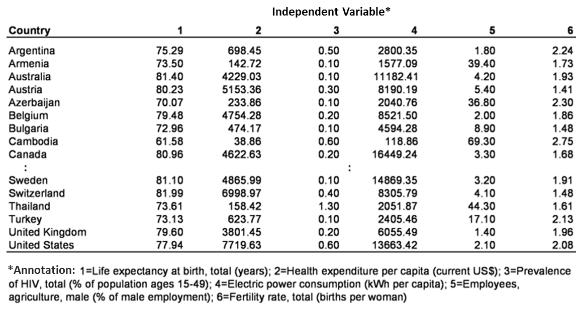
Table 1: World Bank data from the year 2008
In this case, it is not possible to show the data as a diagram because there is more than one independent variable.
The equation of the regression lines with multiple variables is generally shown as follows:
Figure 3: Regression equation
whereby
y = the estimate of the dependent variable
0 = the section of the y axis
k = the slope of the line of variable k
xk = the independent variable k
u = the error term
The example includes the following non-standardized coefficients in the regression equation (see Chapter 3: “Multiple regression with SPSS”):
y = 78,57049 + 0.00067×1 -1,18351×2 + 0,00003×3 – 0.16343×4- 0.74931×5
whereby
y = the life expectancy at birth, total (years)
x1 = the health expenditure per capita (current USD)
x2 = the prevalence of HIV, total (% of population ages 15-49)
x3 = Electric power consumption (kWh per capita)
x4 = Employees, agriculture, male (% of male employment)
x5 = Fertility rate, total (births per woman)
The regression equation with standardized coefficients can be shown as follows:
y = 0.258×1 – 0.538×2 + 0.038×3 – 0.407×4 – 0.073×5
As shown in the equations, the coefficient of the independent variable IV1 (“Health expenditure per capita”) has a positive sign. In other words, countries with above-average per capita expenditures on health services have higher average life expectancy rates than countries where such expenditures are lower. If IV1 (“Health expenditure per capita”) increases by one unit, the dependent variable (“Life expectancy at birth”) will increase by 0.258 units, provided that all other independent variables remain constant (ceteris paribus). The coefficient of the second independent variable IV2 (“Prevalence of HIV”) has a negative sign. The higher the number of persons with HIV symptoms in the various countries, the lower the average life expectancy. The coefficient of the third independent variable IV3 (“Electric power consumption”) has a positive sign. The signs of the coefficients of the fourth independent variable IV4 (“Employees in agriculture”) and the fifth independent variable IV5 (“Fertility rate”) are both negative. A closer look at the size of the standardized coefficients shows that the influence of IV3 (“Electric power consumption”) and IV5 (“Fertility rate”) on the dependent variable is considerably smaller than the influence of the other variables. The coefficients within the same equation can be compared only through the standardization. Considering the above-mentioned regression equation exclusively could lead to the wrong conclusion that IV5 has a larger influence than IV4, and especially than IV1. However, when considering the standardized equation, it becomes clear that IV5 has only a minimal influence on the independent variable.
The coefficients of the different equations can be compared only once the same model has been tested on different samples and the variables have been captured in the same way.
2.3 Testing the regression function
This section tests the quality of the estimate of a particular regression function: The aim is to find out how good the model really is, which involves calculating the coefficient of determination R2 and the F-statistic.
2.3.1 The coefficient of determination R2
The coefficient of determination R2 is the first quality measure. It shows the ratio between the explained variance and the entire variance and indicates how well the regression line fits with the empirical data.
The quality of the model is not expressed as the R2 value but as the corrected R2 value from SPSS, which includes the number of predictors. An increase in the number of predictors will artificially increase R2, which also increases through the assumption of insignificant regressors and therefore will never become smaller.
The R2 value is always between 0 and 1. In the case of a perfect linear correlation, R2 equals 1 and the model thus explains the entire variance. The smaller the value, the less of the variance can be explained through the equation.
In the example, the corrected R2 value is 0.772 (see Chapter 3: “Multiple regression with SPSS”), which means that the model can explain 77.2% of the variance.
According to Cohen (1992) the sizes of the effect are as follows:
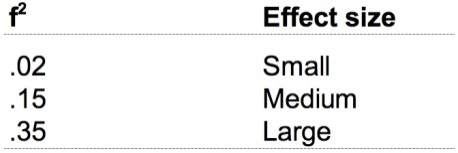
Table 2: Effect sizes according to Cohen (1992)
whereby the following formula describes the relationship between f2 and R²:
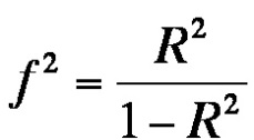
Figure 4: Equation for R2
The R2 values according to Cohen (1992) are as follows:
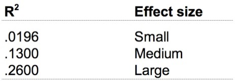
Table 3: Effect sizes in R2 according to Cohen (1992)
An R2 value of 0.772 would indicate a large effect size.
0.1.1.1.2 2.3.1 F-statistic
The F-statistic indicates whether the coefficient of determination R2 came about by chance. This also considers the scope of the sample. This involves an analysis of variance that calculates the ratio of the explained variance (regression) to the unexplained variance (residuals).
For this example, SPSS produces an F-value of 47.601 and a significance (p-value) of .000 (see Chapter 3: “Multiple regression with SPSS”). This value is less than .050 and therefore significant. It can be assumed that the correlation of the variables did not come about by chance.
2.4 Testing the regression coefficients
This section tests the independent variable’s contribution to the model as a whole.
Table 4 gives an overview of the variables, the associated regression coefficients, and the significance levels. The coefficients are important for estimating the influence of the different variables. In some cases, it makes sense to remove certain independent variables from the model (“stepwise regression”) once the coefficients have been tested:
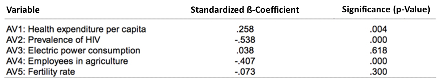
Table 4: Regression coefficients of the example data (IV: Life expectancy at birth)
If the output p-value is less than .050, it can be assumed that the regression coefficient is significant. In this example, this does not apply to the third independent variable IV3 (“Electric power consumption”) and the fifth independent variable IV5 (“Fertility rate”). It therefore makes sense to remove these variables from the model. Based on this example is becomes clear that although the model as a whole may be significant, it nevertheless is important to consider the individual regression coefficient separately.
Removing certain variables from the model will change the regression coefficient of the other variables.
2.5 Testing the model prerequisites / residuals analysis
This section explains how to test for autocorrelation among the residuals and ensure that there is no multicollinearity. Once the validity criteria have been met it is possible to interpret the model in terms of its content. If this is not the case, the model must be refused.
2.5.1 Heteroscedasticity
Carrying out the regression analysis also presupposes that the residuals of the data have the same variance. This condition is referred to as homoscedasticity, which can be tested by considering the residuals. In SPSS, the following diagram can be created from the example data:
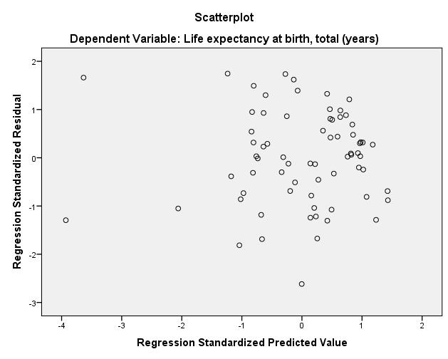
Figure 5: Testing for homoscedasticity
The x-axis shows the regression of the standardized estimated values of the dependent variable; the y-axis shows the standardized residuals. Heteroscedasticity is given when the diagram indicates that a relationship exists between the two variables or that a certain pattern can be discerned. Since this is not the case here, it can be assumed that homoscedasticity is given.
2.5.2 Autocorrelation
Carrying out a regression analysis also presupposes that there is no correlation between the residuals. In SPSS, it is possible to test for an autocorrelation by means of the Durbin-Watson test,
which can assume values between 0 and 4. Here, the following applies: A value of 0 indicates a fully positive autocorrelation, a value of 2 indicates no autocorrelation, and a value of 4 indicates a fully negative autocorrelation.
For the example data, SPSS produces a Durbin-Watson value of 2.011 (see Chapter 3: “Multiple regression with SPSS”) and it can therefore be assumed that autocorrelation is not given.
2.5.3 Multicollinearity
A multiple regression requires the absence of multicollinearity; in other words, independent variables may not be expressed as a linear function of another independent variable. Empirical data usually have some multicollinearity; however, it should not be too strong.
Very strong multicollinearity can result in the regression becoming significant, yet none of the regression coefficients would reach such a result when considered individually. In this case, regression coefficients of the independent variables could also change a great deal if others are included in or removed from the model.
The correlation matrix of all independent variables can serve as an initial indicator of multicollinearity. However, because this matrix can show correlations only in pairs, it is not possible to exclude multicollinearity entirely.
In SPSS, two statistics can be calculated for testing the variables for multicollinearity: The tolerance value and the variance inflation factor. The tolerance value is used for estimating if any linear dependencies with other predictors exist and is calculated as follows:
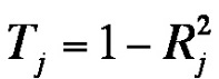
Figure 6: Tolerance value
whereby
= the coefficient of determination of the regression of independent variables Xj on the independent variables of the regression function
The variance inflation factor is the reciprocal of the tolerance value:
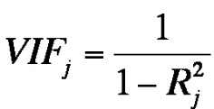
Figure 7: Variance inflation factor
The literature describes the following rule of thumb: The tolerance value should not be below 0.10, and the variance inflation factor should not be above 10. According to these authors, multicollinearity is not given if the values are below or above these thresholds. When conducting a regression analysis, SPSS does not include multicollinearity. If multicollinearity is given, it makes sense to recalculate the regression analysis by including only the desired variables.
For this example, the tolerance values are between 0.434 and 0.857, and the variance inflation factor values are between 1.1167 and 2.306 (see Chapter 3: “Multiple regression with SPSS”). It can therefore be assumed that multicollinearity is not given.
2.6 Selecting the regression model
This example shows that the available variables provide several options for calculating the regression equation.
For example, a certain variable could be excluded from the equation, which would then be calculated with only 3 or 2 independent variables. It therefore follows that additional variables also allow for a greater number of possible models.
The default settings in SPSS factor all the independent variables into the regression equation (see the “Linear Regression” dialogue box under “Method: Enter”). In SPSS, it is of course possible to calculate all the possible equations and compare the respective models; however, more variables also mean more work. SPSS offers several possibilities for a simpler comparison of multiple models, for example conducting a stepwise regression analysis (see “Linear Regression” under “Method: Stepwise” in SPSS dialogue box), whereby the variables are included in the model successively.
Here, first the independent variable that has the highest bivariate correlation with the dependent variable is included in the model, followed by the variable with the second highest correlation, and so on – until there is no more variable with a significant correlation.
It may happen that SPSS suggests a particular model for the best possible solution; however, this may not be justifiable for theoretical or content-related reasons because it involves a mathematical analysis. In such cases, it makes sense to opt for a “mathematically” imperfect model, even if it means not being able to explain the same amount of the variance.
SPSS allows also for blocks of independent variables to be included in the regression equation successively. For example, IV1 (“Health expenditure per capita”) and IV2 (“Prevalence of HIV”) can be added as Block 1, followed by IV3 (“Electric power consumption”), IV4 (“Employees in agriculture”), and IV5 (“Fertility rate”) as Block 2. At the same time, every variable can also be included as a separate block. SPSS first produces the regression equation and associated values for Block 1, then for all variables from Block 1 and 2 together, then for Block 1, 2 and 3, etc., making it possible to see how the regression equation and values change when one variable is or several variables are added to the model. By selecting “R squared change” (under “Statistics”), SPSS indicates the increase in the R-square that the additional variable and/or the additional block of variables bring to the model.
Furthermore, it indicates whether the increase is significant. The sequence in which the variables or blocks are added can be determined manually. It makes sense to first include the variables in the blocks that can be best justified theoretically.
Within the blocks, however, it is possible to select the method freely. For example, in the case of 6 independent variables it is possible to first include 3 variables with SPSS’s “Enter” method jointly in the equation, then 3 variables with SPSS’s “Stepwise” method, allowing for comparisons of different types and models. But here, too, there should be a plan for how to proceed, because only models that are sound with respect to theory and content should be selected.
3. Multiple regression with SPSS
SPSS calculates a regression equation even if the prerequisites for the regression analysis are not met. Before interpreting the content of a regression analysis, it is essential to ensure that all the prerequisites have been met correctly.
3.1 Model with five independent variables
The following figures are of the SPSS output of the mentioned example.
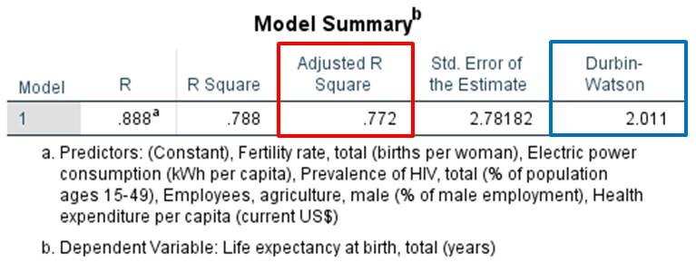
Figure 8: Coefficient of determination and the Durbin-Watson statistic
The column marked red in Figure 8 shows the corrected R2 value, and the column marked blue shows the Durbin-Watson statistic. The corrected R2 value of the model is 0.772. The model explains 77.2% of the variance of the dependent variable (“Life expectancy at birth”).
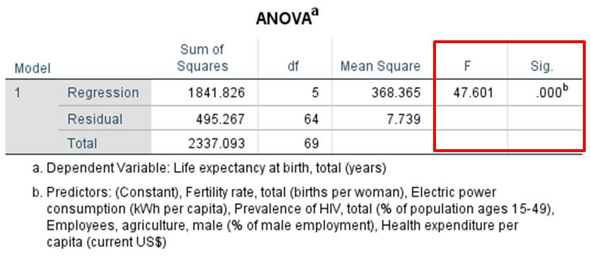
Figure 9: F-statistic with p-value
Figure 9 shows the F-value and the associated significance level. The F-test indicates that the model as a whole is statistically significant.
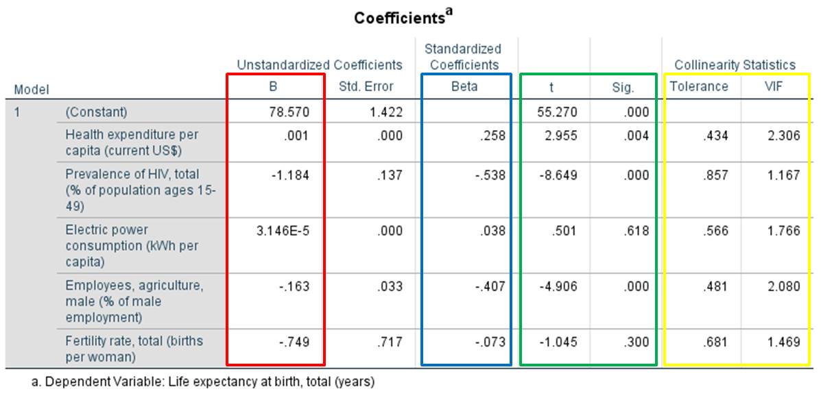
Figure 10: Regression coefficients, p-values, tolerance values, and variance inflation factor values
Figure 10 shows the regression coefficients of the regression lines and the standardized regression equation.
The value labeled as “Constant” in the column marked red refers to the intersection with the Y axis. The column marked red also shows the slopes of the individual variables. The column marked blue has the standardized regression coefficients. The standardized line does not intersect the Y axis and therefore also has no value under “Constant.” The green column shows the p-values of the regression coefficient. The column marked yellow shows the tolerance and the variance inflation factor values for testing for multicollinearity.
3.1 Model with three independent variables
The following figures are taken from the SPSS output for the model with only three variables. The independent variables IV3 (“Electric power consumption”) and IV5 (“Fertility rate”) have been removed from the model because of the non-significant regression coefficient.
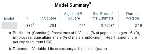
Figure 11: Coefficient of determination and Durbin-Watson statistic (example with 3 independent variables)
Figure 11: Coefficient of determination and Durbin-Watson statistic (example with 3 independent variables)
Figure 11 has 0.774 as the corrected R2 value for the model. The model explains 77.4% of the variance of the dependent variable (“Life expectancy at birth”).
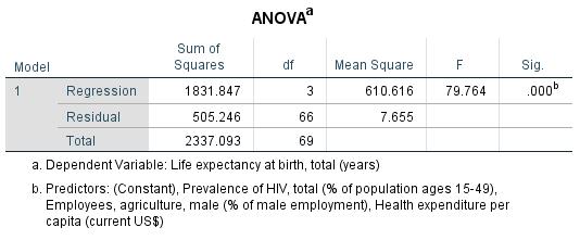
Figure 12: F-statistic with p-value (example with 3 independent variables)
The F-test in Figure 12 shows that the model with three independent variables as a whole is statistically significant.
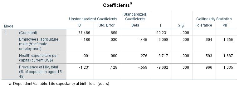
Figure 13: Regression coefficients, p-values, tolerance values, variance inflation factor values (example with 3 independent variables)
Figure 13 indicates that all regression coefficients are significant in the model with three independent variables.
4. SPSS commands
SPSS dataset: Example dataset used for the Multiple-Regression.sav
Click sequence: Analyze > Regression > Linear > Define dependent and independent variables
Syntax: REGRESSION
Multicollinearity: In the regression window, select “Statistic” > “Collinearity diagnosis”
Autocorrelation: In the regression window, select “Statistic” > “Durbin-Watson”
Diagram of heteroscedasticity: In the regression window, select “Diagrams” > *ZRESID on the y-axis, *ZPRED on the x-axis
5. Literature
Cohen, J. (1992). A power primer. Psychological Bulletin, 112, 155-159.