
1. Introduction
2. Procedure
3. Correlation with SPSS
4. SPSS commands
5. Literature
1. Introduction
A correlation analysis provides information about a statistical correlation between two interval scaled attributes (LINK to scale levels). Because this involves two variables, the term “bivariate correlation” is used. A correlation analysis should be chosen over a simple linear regression analysis whenever the assumed direction of the correlation cannot be determined.
1.1. Possible problem formulations
The correlation analysis is suitable for questions that examine a correlation between two attributes, such as “Is there a correlation between age and political orientation?” or “Do working hours and income correlate?”
2. Procedure
The steps for calculating a bivariate correlation can be explained based on a question taken from the field of human resources.
Data about a person’s motivation level is obtained through a standardized test that was conducted during a research project. The resulting motivation index can assume values between 0 and 20. Furthermore, various measured values (e.g. salary, rate of promotion, etc.) were used for compiling an index with values ranging between 0 and 100 for gauging a person’s professional success. Both variables can thus be interpreted as being interval scaled. The research question can be formulated as follows:
Is there a correlation between motivation and success?
The purpose of the inquiry is to find out if a person’s motivation and success at work are somehow related.
2.1 Hypothesis formulation
To test the research question statistically, it is necessary to formulate hypotheses. In this case formulating the hypotheses raises the question about the correlation between “Success” and “Motivation.” While it can be assumed that a person’s motivation is the cause of his or success at work, the opposite may apply as well: success at work can equally be the source of motivation.
The null hypothesis and the alternative hypothesis are as follows:
H0: r = 0 The correlation coefficient equals zero.
HA: r ≠ 0 The correlation coefficient does not equal zero.
To test the hypothesis, it is first necessary to obtain data. The following Table 1: “Example data” contains the data of 12 test subjects.
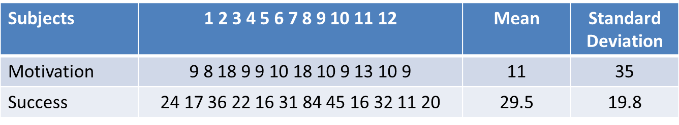
Table 1: Example data
The scatter plot indicates that a linear correlation exists between the variables of “Success” and “Motivation.”
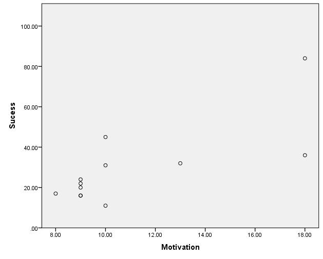
Figure 1: Scatter plot
2.2 Calculating the correlation coefficient
When calculating the correlation coefficient r it is assumed that a linear and non-directional correlation exists between the two variables.
Note: The correlation coefficient r is also referred to as product-moment correlation, Pearson correlation, Pearson-Bravais product moment correlation, or Bravais-Pearson correlation.
The correlation coefficient r is calculated by dividing the covariance (cov(x,y)) of two variables (x,y) by the product of the standard deviations of the variables (sx, sy). Because of this division, the correlation coefficient becomes invariant vis-à-vis a change in the scale or a linear transformation, and it can take a value between -1 and 1.
2.3 Conducting the hypothesis test
The correlation coefficient allows for drawing a conclusion about the nature of the correlation. However, it is necessary to conduct a hypothesis test to also establish if a correlation exists in the population. In the case of the correlation coefficient, the t-test is used for testing the hypothesis of whether the correlation coefficient differs significantly from 0.
Prerequisite data: Conducting the t-test presupposes normal distributed variables. Exception: One of the two variables is a dummy variable (2 categories).
Whether a correlation coefficient is significant depends on the size of the sample, among other things. For example, in a large sample, a smaller r value is sufficient for becoming significant than would be the case in a large sample. If a correlation coefficient is significant, the question arises as to whether the results are also of practical relevance. Here, the measure of the effect size is useful because it makes it possible to draw conclusions about the practical relevance of a significant test result and because it is virtually unaffected by sample size n.
The correlation coefficient r as a standardized measure is generally used for gauging the effect size. According to Cohen (1992) and Field (2009: 170) the following values apply during a correlation analysis to draw conclusions about the effect size, whereby the +/- sign indicates the direction of the correlation (see Table 2: Effect sizes).
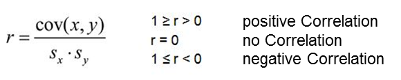
Table 2: Effect sizes
The coefficient of determination R2 describes the explained proportion of the variance of the data (see Table 3: Coefficient of determination).
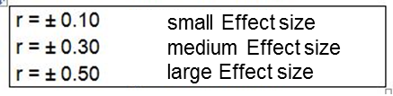
Table 3: Coefficient of determination
3. Correlation with SPSS
SPSS automatically produces the p-value (referred to as “Sig.” in SPSS) when calculating the correlation.
Note: The dialogue box also offers the option of marking significant correlations. However, it must be noted that SPSS may require a different significance level. The values should therefore be checked again and compared with the defined significance level.
The table generated in SPSS shows the correlation and the p-value (see Figure 2: SPSS output of the example data):
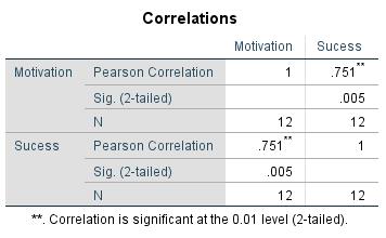
Figure 2: SPSS output of the example data
“Success” and “Motivation” correlate with a p-value of .005. If a significance level of α = .050 is given, the null hypothesis can be refused, which means accepting the alternative hypothesis according to which the correlation coefficient is unequal to 0. For the example data, SPSS produces a correlation coefficient of .751. It can therefore be assumed that a positive linear correlation exists between “Motivation” and “Success.” An r of .751 also indicates a large effect (see Table 2: Effect sizes). Squaring the correlation value r produces an r² value of .564. 56.4% of the data’s variability can be explained by the model.
Note regarding Figure 2: The correlation coefficient of 1 in the diagonal can be explained through the correlation of the variable with itself.
4. SPSS commands
Click sequence: Analyze > Correlation > Bivariate
(Select “Pearson” in the dialogue box)
Syntax: CORRELATION