1. Introduction
2. Procedure
3. Chi-square contingency analysis with SPSS
4. SPSS commands
5. Literature
1. Introduction
Pearson’s chi-square test of independence is a non-parametric statistical procedure with a chi-square-distributed test statistic that is used for testing the mutual dependency of two attributes. The chi-square contingency analysis is an extension of the “classical” cross-table test that examines each of two attributes against two characteristics.
Here, cross tables can be used for calculating the various coefficients that reflect the size and direction of the correlations.
2. Procedure
This chapter explains in detail the procedure of the chi-square contingency analysis based on the following question:
Is there a correlation between age and the likelihood of getting intestinal cancer?
The procedure of the chi-square contingency analysis is summarized in three steps, which are described in the following section.
2.1 Schematic representation
The question is examined based on a dataset provided by the Statistical Analysis Institute (SAS). The data is on 406 persons who had a colonoscopy (intestinal screening).
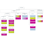
The answer to the questions can be found with the help of a schematic representation, which in this case looks as follows:
Figure 1: Schematic representation
This example uses the variables “Intestinal cancer result” (0 = “negative result”; 1 = “small adenoma; 2 = large adenoma) and “Age” (1 = 30-39 years; 2 = 40-49 years; 3 = 50-59 years; 4 = 60-69 years; 5 = 70-79 years).
2.2 Calculating the coefficients
It is possible to calculate various coefficients that reflect the size and direction of the relationships. Three of these coefficients are described in the following section.
Figure 2 shows how frequently the attribute categories of the two variables being tested occur.
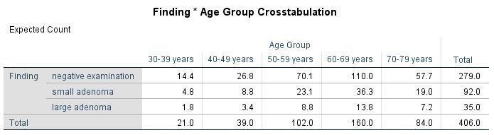
Figure 2: Cross table of the example data
The chi-square test statistic is calculated by comparing the table of observed frequencies with the table of expected frequencies in the case of statistical independence. The values of the table of expected frequencies are calculated by means of the marginal distributions (totals across rows and columns, see “Total” in Figure 3). The marginal distributions correspond with the estimated probability distributions of the groups under the null hypothesis.
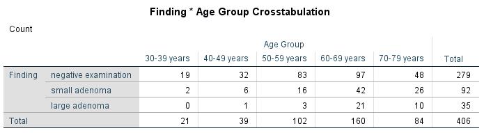
Figure 3: Table of expected frequencies
The chi-square test examines the extent to which the observed values (see Figure 2) deviate from the statistical independence (see Figure 3). The chi-square test statistic is calculated as follows:
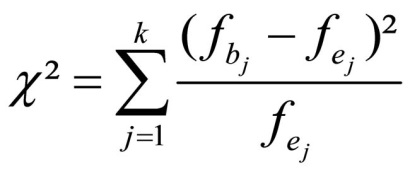
Figure 4: Calculating the chi-square test statistic
whereby
k = the number of cells
fb = the observed absolute frequency within cell j
fe = the expected absolute frequency within cell j
The calculated chi-square test statistic is afterwards tested for significance.
The chi-square value always has a positive sign and depends on the number of groups. The chi-square test serves exclusively for finding out whether a relationship exists between the variables being examined. There are several standardized correlation measures that are based on the chi-square test statistic. These coefficients are then used for determining the size and direction of the correlation. Standardizing causes the values from the calculated correlation measures to be between 0 and 1.
The coefficient of Cramer’s V can be used as an initial option for standardizing and is calculated as follows:
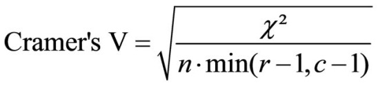
Figure 5: Calculating Cramer’s V coefficient
whereby
n = sample size
r = the number of rows
c = the number of columns
The expression “min(r-1, c-1)” means that the number of rows and columns is reduced by 1 and the smaller of the two values is used in the equation. Cramer’s V can also be useful when comparing several correlations between variables with each other.
Pearson’s contingency coefficient can be used as a second option for norming and is calculated as follows:
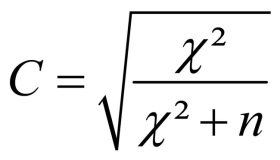
Figure 6: Calculating Pearson’s contingency coefficient
whereby
n = sample size
The upper limit of C is determined as follows:
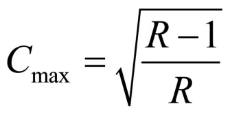
Figure 7: Calculating Pearson’s contingency coefficient
Figure 7: Calculating Pearson’s contingency coefficient
whereby
R = min (r, c)
r = the number of rows
c = the number of columns
Pearson’s contingency coefficient serves only for comparing tables with the same number of rows and columns.
The following coefficients are calculated for the example data:
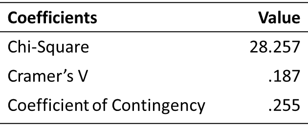
Table 1: Coefficients of the example data
2.3 Testing for significance
This section examines the test statistic for significance. The calculated chi-square value is compared with the critical value of the chi-square distribution as determined by the degree of freedom. If the calculated value is greater than the critical value, a significant relationship can be assumed. Table 2 provides an overview of the calculated p-values:
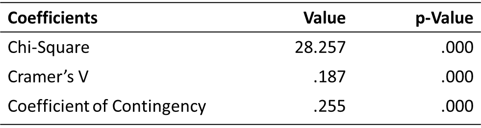
Table 2: P-values of the coefficients of the example data
Because the p-value of the Chi Square coefficient is smaller than the significance level of .050, a correlation exists between the tested variables of “Intestinal cancer result” and “Age.”
The p-values of the Cramer’s V coefficient as well as Pearson’s contingency coefficients are also below significance level of .050. Because Cramer’s V coefficient is smaller than .300, the variables being tested indicate a very weak correlation.
2.4 Prerequisites for a chi-square test
Conducting the chi-square distribution test requires three prerequisites, which are described in the following section.
Firstly, the sample size must be at least 50. If the sample size is between 20 and 50, it is necessary to correct the chi-square according to Yates (in this case, SPSS performs a “Continuity correction” automatically if there are two variables with two characteristics). If the sample size is smaller than 20, the exact Fisher test should be used instead of the chi-square test.
Secondly, the expected frequencies in all the cells of the cross table must be greater than 5. If this prerequisite is not met, the exact Fisher test should also be used instead of the chi-square test.
Thirdly, the degrees of freedom v = (r – 1) • (c – 1) should be greater than 1. The “classical” cross-table test that examines each of two attributes with two characteristics does not meet this prerequisite. In this case, the Chi Square needs to be corrected in accordance with Yates.
In this example, the second prerequisite is not met. However, because the two variables have more than two characteristics and not more than 20% of the expected frequencies are less than 5, the chi-square test can be carried out nevertheless.
3. Chi-square contingency analysis with SPSS
SPSS produces the following figures when performing the chi-square contingency analysis:
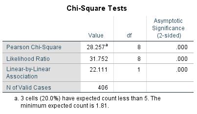
Figure 8: Chi-square test statistic
Figure 8 shows the Pearson’s chi-square test statistic and the associated p-value. The output p-value is less than .050. There is a relationship between age and the likelihood of getting intestinal cancer.
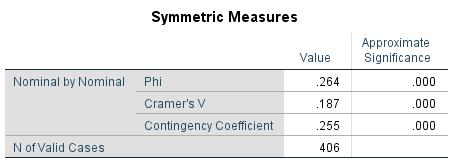
Figure 9: Cramer’s V and contingency coefficient
Figure 9 shows Cramer’s V coefficient and the contingency coefficient as well as the associated p-values. Because the coefficients are significant and positive, there is a positive correlation between the occurrence of intestinal cancer and age.
4. SPSS commands
SPSS dataset: Example dataset used for the Chi-Quadrat-Unabhängigkeitstest.sav
Click sequence: Analyze > Descriptive statistics > Cross tables
Syntax: CROSSTABS TABLES