
1. Introduction
2. Procedure
3. Logistic regression with SPSS
4. SPSS commands
5. Literature
1. Introduction
Logistic regression analyses are generally used when developing a model for the probability of a certain event occurring based on the characteristic of one or several independent variables. The independent variables can have any scale level and do not need to be uniform within an equation. A binary logistic regression is used in cases where the dependent variable is dichotomous (with two characteristics). Multinomial logistic regressions are used when there is a nominal scaled dependent variable with more than two categories. When the dependent variable is ordinal scaled and has more than two categories, it is possible to calculate an ordinal logistic regression. This chapter only covers the binary logistic regression, which in applied research is used most frequently in logistic regression analyses.
2. Procedure
This chapter explains in detail the procedure of a logistic regression analysis based on the following question:
Which variables influence the probability of survival among patients admitted to an intensive care unit?
This example uses a binary logistic regression to examine the influences of several independent variables on the dichotomous variable of “vital status” (with the two levels “lived” and “died”). The point is to determine the probability of a particular event occurring rather than to estimate the specific value of a dependent variable, as in the case of linear regression analysis.
The procedure for conducting a logistic regression analysis is summarized in five steps, which are described in the following section.
2.1 Model formulation
In the example, the dependent variable is dichotomous and can assume two levels: 0 (“Lived”) or 1 (“Died”). Figure 1 shows a possible distribution of an independent and a dependent variable.
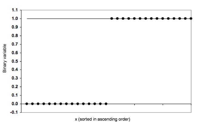
Figure 1: Example distribution
Figure 2 shows an attempt to include the displayed data of a regression line.
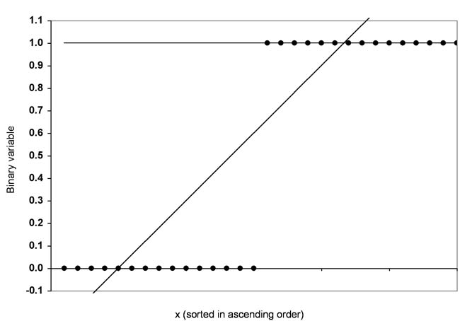
Figure 2: Example distribution with a regression line
Figure 2 shows an attempt to insert a regression line into the data. For example, the line also crosses values that are greater than 1 and smaller than 0. Instead of a regression line, it makes sense to use a logistic function to fit the data shown. The logistic function can assume only values between 0 and 1. Figure 3 shows the logistic function for the example distribution:
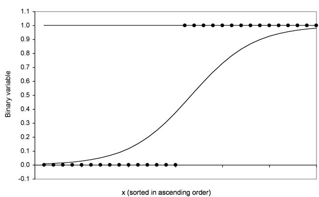
Figure 3: Example distribution with logistic function
The logistic function provides the probability of occurrence of an event and not the estimate of the values of the dependent variables. It is calculated with the following equation:
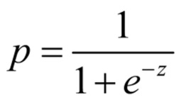
Figure 4: Logistic function
whereby
p = the probability
e = Euler’s number (approx. 2.718)
Variable z is defined with the following equation:
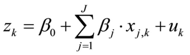
Figure 5: Logistic regression equation
whereby
k = the case
β = the coefficients
j = the number of independent variables
xj,k = the characteristics of independent variable j for case k
uk = the error term
The z-values are also referred to as “logits” and the coefficients as “logit coefficients.” The logit coefficients reflect the size of the influence of the independent variables.
To formulate a model for calculating a logistic regression it is generally first necessary to determine which factors could influence the probability that the event being examined occurs. Examining the question of the example therefore first means determining the factors that could influence the probability of living or dying among patients who are admitted to the intensive care unit.
The question is examined based on a dataset from Hosmer & Lemeshow (2000), which contains many variables. For didactic reasons, 10 variables were selected by means of a prior process, and they are included in the model. The sample includes 200 persons who were admitted to the intensive care unit.
The resulting model looks as follows:
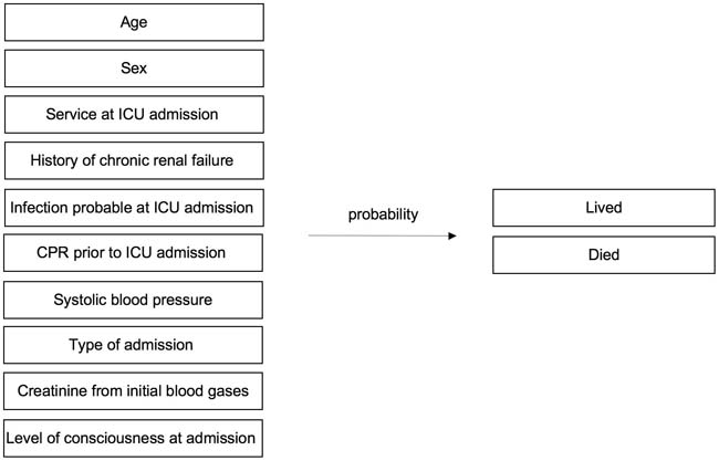
Figure 6: Example model Note: ICU = intensive care unit; CPR = cardiopulmonary resuscitation
The example model includes the following variables: The first independent variable is the age and is interval scaled. The second independent variable is the gender. The third independent variable is the “Service at intensive care unit admission” with the levels “medical” or “surgical.” The fourth (“History of chronic renal failure”), fifth (“Infection probable at ICU admission), and sixth independent variable (“Cardiopulmonary resuscitation prior to ICU admission”) are dichotomous with the levels of “no” or “yes.” The seventh independent variable is the systolic blood pressure (in mm Hg), which is interval scaled. The eighth independent variable (“Type of admission”) has the levels “Selective” or “Emergency.” The ninth independent variable (“Creatinine from initial blood gases”) has two levels, which are defined through a cut-off value of the creatinine values. The tenth independent variable (“Level of consciousness at admission”) has the levels “No coma or stupor,” “Deep stupor,” or “Coma.”
2.2 Estimating the logistic regression function
This section explains how to estimate a particular regression function based on empirical data. In a logistic regression, the estimate is derived from a logarithmic likelihood function. In the example, SPSS produces the following equation for z:
z = -3.98 + 0.03×1 – 0.25×2 – 0.11×3+ 0.44×4+ 0.20×5 + 0.55×6 – 0.01×7 + 1.84×8 + 0.55×9 + 1.74×10
whereby
z = the logit
x1 = the patient’s age in years (AGE)
x2 = the patient’s sex (SEX)
x3 = the service at ICU admission (SER)
x4 = the history of chronic renal failure (CRN)
x5 = the infection probable at ICU admission(INF)
x6 = the cardiopulmonary resuscitation prior to ICU admission (CPR)
x7 = the systolic blood pressure at ICU admission in mm Hg (SYS)
x8 = the type of admission (TYP)
x9 = the creatinine from initial blood gases (CRE)
x10 = the level of consciousness at admission (LOC)
The regression coefficients or logit coefficients reflect the strength of the independent variable’s influence on the likelihood with which the event could occur (in the example: Probability that patients will die).
2.3 Interpreting the regression coefficients
The regression coefficients of a logistic regression cannot be interpreted in the same way as the coefficients of a linear regression analysis (for example, “if independent variable X1 increases by 1, dependent variable will increase by β1”). In the case of a logistic regression analyses, the independent and the dependent variables do not have a linear correlation, i.e. the effect of the independent variable varies above the value range: An increase in the independent variable X1 from 1 to 2 can have a different effect onto the dependent variable than an increase from 3 to 4. Furthermore, the logit coefficients of the independent variables cannot be compared among each other.
In the case of a logistic regression, negative regression coefficients will reduce the relative probability of the event occurring if the x values increase, while positive regression coefficients will increase the relative probability of the event occurring.
Logistic regressions do not interpret the coefficients directly, but only the odds (probability ratios). These are the quotients of the probability of occurrence for an event (y = 1) and of the counter probability (y = 0). The odds are calculated with the following equation:
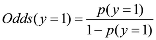
Figure 7: Calculating the odds
whereby
p(a) = the probability of occurrence for event a
The following relationship applies to a logistic regression:
Figure 8: Logit calculation
The logits of a logistic regression constitute the logarithmic odds. The odds ratio refers to the relationship between two odds. When calculating a logistic regression, SPSS produces the odds ratio for every variable. These are labeled as “Exp(B).” Unlike in the case of the logit coefficients, the odds ratios of independent variables can be compared with each other.
The literature generally suggests the following interpretation of the regression coefficients:
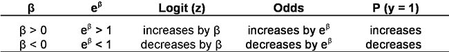
Table 1: Interpretation of coefficients of a logistic regression
In the example, SPSS produces an odds ratio 1.03 for the independent variable “Age” (see Chapter 3: “Logistic regression with SPSS”). A patient who is admitted to the intensive care unit and is one year older than a reference patient will therefore on average have an approximately 3% smaller relative chance of surviving. The odds ratio of the independent “Type of admission” variable is 6.29. This value can be interpreted as follows: Seen statistically, patients admitted to the intensive care unit for emergency treatment have a 6.29 times greater relative probability of dying than patients who came of their own initiative.
2.4 Testing the model as a whole
Once the logistic regression function has been calculated, the model needs to be tested. Here it is important to ensure that the data sufficiently represents the model. The model as a whole needs to be tested based on the -2LL value (twice the “-Log Likelihood”). SPSS first calculates a basic model in which only the constants are included and all regression coefficients are equal to 0. In the next step, the model is calculated with all the variables. SPSS shows the -2LL values of both models as well as the difference between the two values. This difference is then tested for significance with the Chi² test.
In the example, SPSS produces a -2LL value of 200.16 for the basic model and a -2LL value of 146.36 for the model with all the variables (see Chapter 3: “Logistic regression with SPSS”). The value of the difference is 53.80, which is significant (p-value less than .05). At least one of the regression coefficients of the independent variables is therefore unequal to 0.
In the case of a logistic regression, R² (also referred to as “Pseudo-R²”) is an attempt to quantify the variance of the dependent variable as explained based on the independent variables. Although it is calculated differently, R² is interpreted the same way as the coefficient of determination R² of the linear regression. For the example data, SPSS produces a Nagelkerke R² of .373 (see Chapter 3: “Logistic regression with SPSS”). The Nagelkerke R² can assume values between 0 and 1. The literature mentions values above .5 as being very good. The Nagelkerke R² of .373 in the example indicates that the variance of the dependent variable through the independent variable cannot be fully explained.
2.5 Testing the variables
The statistics mentioned in section 2.4 are used for testing whether the model as a whole is adequate for describing the data. In this case, a significant event indicates that at least one of the regression coefficients of the variables being tested is greater than 0. The next step involves testing the coefficients individually for significance.
For this, SPSS produces the Wald statistic, which tests the null hypothesis according to which the individual regression coefficients of the independent variables are equal to 0. The Wald statistic is calculated with following equation:
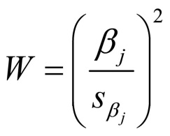
Figure 9: Calculation of the Wald statistic
whereby
j = the index of the independent variables
βj = the regression coefficient
sβ = the standard error of the regression coefficient
The calculated Wald statistic constitutes the squared regression coefficient divided by the standard error, and it is tested for significance with the Chi² test. The Wald statistics with the p-values of the independent variables of the example are shown in paragraph 3 (“Logistic regression with SPSS”) of Figure 16.
3. Logistic regression with SPSS
When calculating a logistic regression, SPSS produces the following figures, among other things:
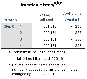
Figure 10: -2LL value of the basic model
Figure 10 “Iteration protocol” for the “Initial block” shows the -2LL-value for the basic model without independent variables.
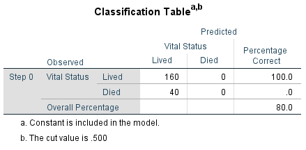
Figure 11: Classification table of the basic model
Figure 11 shows the classification table of the basic model without considering the independent variables.
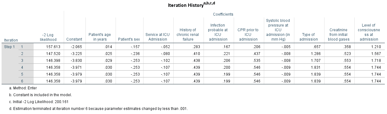
Figure 12: -2LL-values and regression coefficients of the various steps
Figure 12 shows the -2LL-values for the model with all variables. Furthermore, it shows the values of the regression coefficients of all variables, which were calculated in six steps, whereby the lowest row is relevant. Here the regression coefficients of the last step are shown.
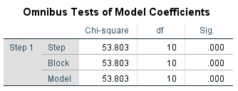
Figure 13: Significance for the model as a whole
Figure 13 shows the “Omnibus test of the model coefficients,” indicating if the model as a whole is significant. The independent variables were introduced into the model blockwise. All the values in the table are therefore identical.
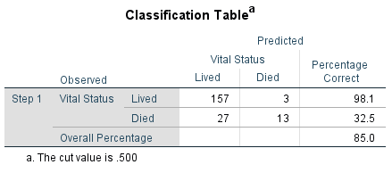
Figure 14: Classification table of the model.
Figure 14 shows that 85.0% of the patients can be classified correctly with the model in terms of the dependent variable. The patients who survived could be allocated more accurately (98.1% correct) than the patients who died (32.5% correct). The value of 85.0% for correctly allocated patients is above the 80.0% shown in the classification table of the basic model (see Figure 11), in which the independent variables were not included. However, the predictive power of the whole model under consideration has improved only slightly (by 5%) compared to the basic model when considering the independent variables.
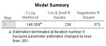
Figure 15: -2LL-value and the Nagelkerke R²
Figure 15 shows the -2LL-value of the model as a whole and of the Nagelkerke R².
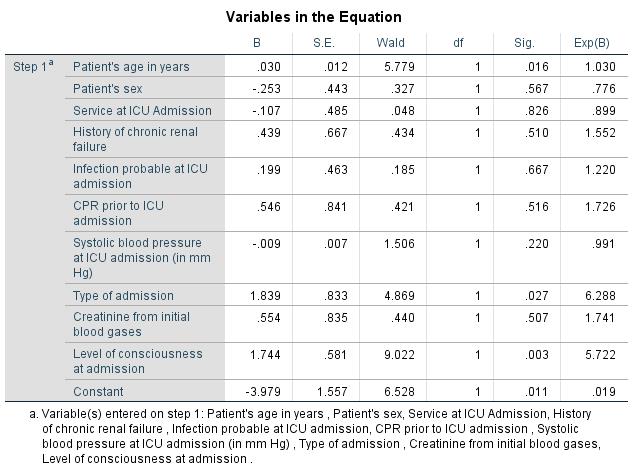
Figure 16: Regression coefficients and the odds ratio
Figure 16 again shows the regression coefficients, the odds ratios, as well as the p-values of all variables. The independent variables of “Age,” “Type of admission,” and “Level of consciousness at admission” have p-values of less than .05. The regression coefficients of these variables are significant. It can therefore be assumed that these independent variables will significantly influence the probability that patients admitted to an intensive care unit will die.
4. SPSS commands
SPSS dataset: Example dataset used for the Logistische-Regression.sav
Click sequence: Analyze > Regression > Binary logistic
Syntax: LOGISTIC REGRESSION
Syntax of the example calculations:
LOGISTIC REGRESSION VARIABLES STA
/METHOD=ENTER AGE SEX SER CRN INF CPR SYS TYP CRE LOC
/PRINT=ITER(1)
/CRITERIA=PIN(0.05) POUT(0.10) ITERATE(20) CUT(0.5).