1. Introduction
Factor analysis is a multivariate analytical procedure used when attempting to carry out a dimension reduction based on assumed correlations among interval scaled variables. The goal is to reduce the variables being tested to a lower number of factors that are as meaningful and independent of each other as possible, and to explain the largest possible part of the variance of the variables in question. A factor analysis can be conducted either as an explorative or a confirmatory procedure. An explorative factor analysis is a procedure conducted only to identify structures, and it is used for generating hypotheses when no assumptions can be made about possible correlations among the variables being examined. The confirmatory factor analysis, on the other hand, is a procedure for testing hypotheses, and it is used when certain correlations can be assumed about the variables that are being examined. This chapter focuses exclusively on the explorative factor analysis.
2. Procedure
This chapter explains in detail the procedure of the explorative factor analysis based on the following question:
Can students’ preferences for six subjects (algebra, biology, calculus, chemistry, geology, and statistics) be summarized in a lower number of factors?
The literature usually summarizes the procedure for conducting an explorative factor analysis into five steps, which are described in the following section.
2.1 Selecting the variables
The first step involves selecting the variables that are to be included in the factor analysis. This means generating a correlation matrix of all the variables. In this example, the factor analysis is conducted by means of a dataset containing the hypothetical answers of 300 students to the question of how much they like their various subjects. The analysis includes six variables (subjects): Algebra, biology, calculus, chemistry, geology, and statistics. Table 1 shows the example dataset:
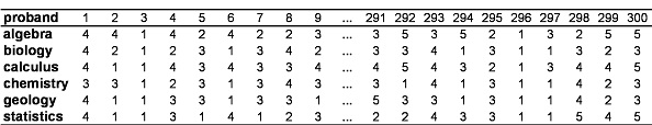
Table 1: Example data
A 5-point Likert scale is used: 1 = “Strongly dislike”, to 5 = “Strongly like”.
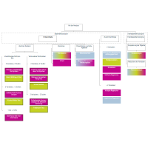
Figure 1 shows the variables being tested, which can, for example, be reduced to two factors. It is not yet possible to know how many factors the different variables being tested can be reduced to (it could also be only one factor, or more than two factors).
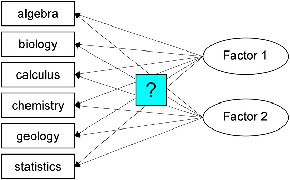
Figure 1: Example of a reduction to two factors
The factors (also referred to as latent constructs) are not measured directly but calculated based on the correlations between the manifest variables being examined.
0.1.1.1.2 2.1.1 Calculating the correlation matrix
A correlation matrix makes it possible to gain an initial overview of the correlations of the variables. This means calculating the bivariate correlations (according to Pearson) of the individual variables. Figure 2 shows the correlation matrix:
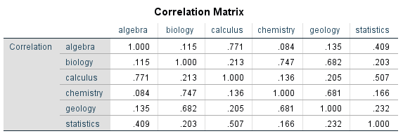
Figure 2: Correlation matrix of the manifest variables
According to Cohen (1988), the effect of a correlation as of .500 can be considered as high. In this example, it thus follows that algebra and calculus, as well as statistics and calculus, have a strong correlation, and that algebra and statistics have a medium correlation. Furthermore, there is a strong correlation between biology and chemistry, between biology and geology, and between chemistry and geology. The correlation matrix, however, is insufficient when determining whether correlated variables can be explained through a common factor. Nevertheless, the variables can be selected already at this stage if some do not correlate, or correlate only slightly, with others and the possibility of allocating a common factor can therefore be ruled out for sure.
0.1.1.1.3 2.1.2 Suitability of the correlation matrix
Raw data is suitable for conducting a factor analysis if the Kaiser-Meyer-Olkin Measure of Sampling Adequacy (KMO) is greater than .60. The KMO assumes values between 0 and 1 and measures how strongly the variables being tested correlate. The size of the KMO value can be evaluated as follows (according to Backhaus, Erichson, Plinke & Weiber, 2006):
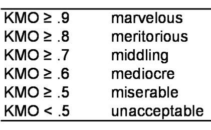
Table 2: Interpreting the KMO value
Another criterion for determining if the data are suitable for a factor analysis is Bartlett’s Sphericity Test, whose working hypothesis states that none of the variables being tested may correlate with each other.
The following table has the Kaiser-Meyer-Olkin Measure of Sampling Adequacy and Bartlett’s Sphericity Test as applied to the example data:
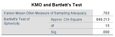
Figure 3: Kaiser-Meyer-Olkin measure of sampling adequacy and Bartlett’s sphericity test
In this example, the KMO value is .703. According to Backhaus, Erichson, Plinke and Weiber (2006), measure of sampling adequacy values above .70 are considered to be middling (see Table 2). The p-value of the Bartlett’s Sphericity Test in this example is significant (p < .001). It can therefore be assumed that the example data is suitable for a factor analysis. In addition, anti-image matrices that rely on the decomposition of the two variances can be used for evaluating whether individual variables should be included in the factor analysis. This means bringing the variance portion of one variable that can be explained with the correlating variables (image) into association with the inexplicable variance portion (anti image). The variables are suitable to include in the factor analysis if the values of the anti-image matrix turns out to be low. Figure 4 shows the anti-image matrices:
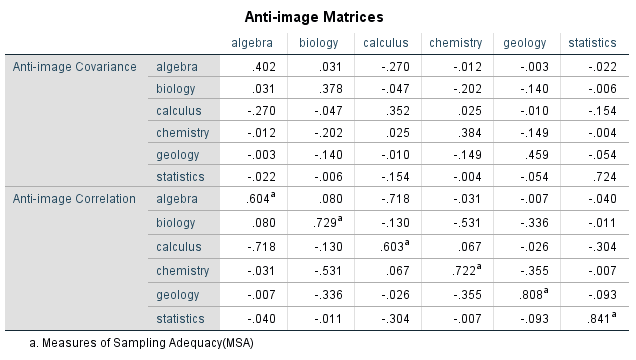
Figure 4: Anti-image matrices
Based on the anti-image matrices, it is possible to determine whether individual variables should be removed from the factor analysis. The values in the diagonal serve as a measure for determining the sample size, and they are marked with a superscripted “a.” Table 2 can be used for evaluating the values. In this example, the anti-image correlation values are between .603 (calculus) and .841 (statistics). It therefore follows that all variables can be included in the factor analysis.
2.1 Determining the communalities
The communalities describe the individual variables’ variance portions that can be explained with the extracted factors (total of the squared loadings of a variable across all factors). There are several procedures for extracting the factors, and they differ in how the communalities are determined. Conducting a principal components analysis assumes that the extracted factors fully explain the variance of the variables. The major axis analysis, on the other hand, is estimated on the assumption that the variables have inexplicable residual variances. This example uses only the calculation from the principal components analysis, which is the most frequently used method. The following figure shows the communalities of the variables of the example data:
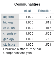
Figure 5: Communalities
A principal components analysis assumes that the variance of every variable included in the analysis can be explained fully (the reason the communalities shown in Figure 5 are initially 1). The second column shows the communalities of the variables being tested after the factors have been extracted.
2.2 Extracting the factors
Carrying out a factor analysis involves calculating the matrices and vectors mathematically to develop a new frame of reference (system of coordinates) with fewer dimensions (axes) in which the analyzed data is embedded as well as possible. This means plotting the factors on the axes. In a two-dimensional framework, the vectors can be displayed in image form (variables being tested). The strength of the correlation between the variables corresponds to the proximity of the associated vectors in the system of coordinates. The stronger the correlation between two variables, the smaller the angle of the associated vectors. For the example data, the vectors can be allocated as follows (angle size is selected randomly):
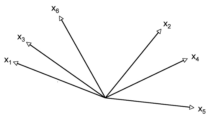
Figure 6: Depiction of the variables as vectors in a system of coordinates
In a principal components analysis, the first factor is laid out so that the largest possible part of the tested variables’ total variance can be explained. In this example, the first axis (first factor) marks the intersection of the six vectors so as to maximize the variance of the vectors to the axis. Orthogonal vectors (with a 90-degree angle) are independent of each other. The goal of a factor analysis is to identify as few independent factors as possible. This is why the orthogonal axis is set first. In a principal components analysis, the second axis (second factor) is set so that it forms a 90-degree angle to the first axis and at the same time maximizes the explained residual variance (see Figure 7). This step is then applied to each further axis that is added. A graphic representation is no longer possible if there are more than two axes.
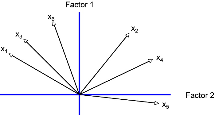
Figure 7: Depiction of the variables as vectors and the factors as axes in the system of coordinates
The size of the angle between a vector and the axis reflects the correlation of the variable and the factor. The larger the factor loading of a variable (correlation of the variable with the factor) the smaller the angle between the vector and the axis (in Figure 7 the angles have random sizes).
2.3 Determining the number of factors
This section explains the two key criteria that can be used when choosing the best possible factor solution. There are no generally valid rules when it comes to determining the ideal number of factors to extract. Based on the Kaiser criterion (in the default settings of SPSS), the factors are deemed relevant if their eigenvalue (portion of the total variance of all variables that can be explained through the factor, i.e. the total of the squared factor loadings across all variables) is greater than one, thus explaining more of the variance than a single tested variable that is included in the factor analysis (Moosbrugger & Schermelleh-Engel, 2007). The following figure shows the table of the eigenvalues of the example data:
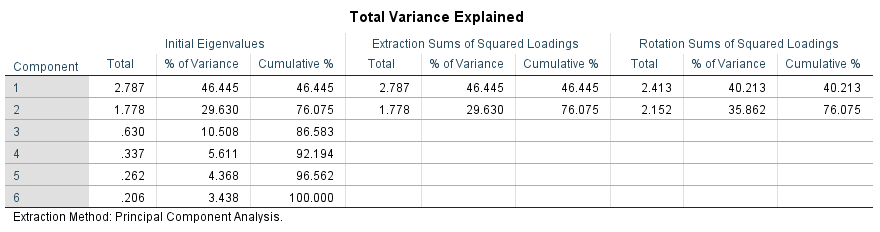
Figure 8: Table of the eigenvalues of the example data
The column labeled “Total” shows the eigenvalues of the factors. In this example, there are two factors whose eigenvalues are greater than one. According to the Kaiser criterion, two factors need to be extracted. These two factors together explain 76.1% of the total (see “Cumulated %” in Figure 8).
Based on the scree test, the relevant factors are those whose eigenvalues lie before the sharp bend in the scree plot (graphic depiction of the progression of the eigenvalues) (Bortz, 1999).
The following figure shows the scree plot of the example data:

Figure 9: Scree plot of the example data
In the case of randomly derived factors, the slope of the scree plot is flat, which is why only the factors above a sharp bend are counted. This example indicates a sharp bend at the third extracted factor (two factors are before the sharp bend). The scree test therefore suggests the extraction of two factors.
Content-related considerations often play an important role in determining the best number of factors to extract. The settings in SPSS allow for extracting more factors than are suggested by the Kaiser criterion.
2.4 Determining the factor values and factor rotation
The next step after determining the number of factors and their extraction involves calculating the size of factor loadings (correlations between the variables being tested and the factors). The following figure shows the factor loadings of the example data:
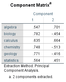
Figure 10: Unrotated factor loadings
In this example, two factors were extracted: The “Component 1” column shows the factor loadings of the first factor (component); the second column shows the factor loadings of the second factor (component). Ideally, every variable correlates strongly with only one factor, which makes it easier to interpret the content of the factors. Usually, however, loadings as of .50 are considered as large. In this example, the components matrix indicates that all variables for the unrotated solution are loaded onto the first factor. Algebra, calculus, and statistics, on the other hand, have a high positive loading onto the second factor, while biology, chemistry, and geology have a negative loading. It is therefore difficult to interpret the factors for this example uniformly with an unrotated solution.
The second step involves rotating the axes. Although this rotation has no effect on the eigenvalues, it causes there to be differences in the loadings. For the example data, the two axes can be allocated as follows:
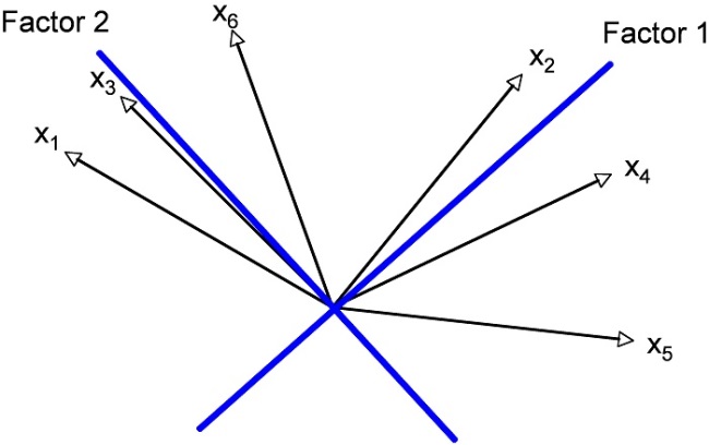
Figure 11: Rotated solution in the system of coordinates
There are two ways of rotating the axes. In the case of a 90-degree rotation (as used in this example), the factors remain independent of each other. In an oblique rotation, the factors depend on each other, i.e. they correlate.
There are numerous 90-degree rotation methods. This example uses the Varimax method, which is most frequently used and results in a reduction of the variables with high multiple loadings. The following figure shows the rotated factor solution:
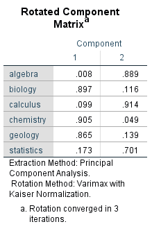
Figure 12: Rotated factor loadings
The rotation in this example makes it possible to find a solution that comes close to a simple structure and in which the variables being tested have very high loadings on one factor and very low loadings on the other factors. The variables of biology, chemistry, and geology have high loadings on the first factor, while algebra, calculus, and statistics have strong correlations with the second factor.
2.5 Factor interpretation
This section interprets the content of factors by searching for general terms for the groups of variables that are loaded onto the respective factor. The interpretation always should be made based on technical considerations as documented in the specialized literature.
In this example, “natural sciences” would work as the general term for the first factor because it has high loadings with biology, chemistry, and geology. The second factor has high loadings with algebra, calculus, and statistics and could therefore be named “Mathematics.” The respective figures would look as follows:
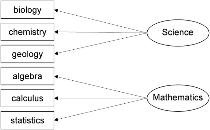
Figure 13: Reduction to two factors
Students’ answers to the question of how much they like algebra, biology, calculus, chemistry, geology, and statistics seem to be influenced by a basic preference for natural sciences or mathematics. Students with a preference for natural sciences, for example, are most likely to choose the subjects biology, chemistry, and/or geology over the subjects algebra, calculus, and/or statistics.