1. Introduction
2. Procedure
3. SPSS commands
4. Literature
1. Introduction
A cluster analysis is a multivariate procedure used for subdividing a certain quantity of objects into groups or “clusters.” Clusters are formed by including several attributes (dimensions) simultaneously, and they can have any scale level. Objects allocated to a particular cluster should be as similar (homogeneous) to each other as possible and differ as much as possible from those allocated to other clusters.
2. Procedure
This chapter explains in detail the procedure of conducting a cluster analysis based on the following question:
Can students be allocated to groups based on their experience with computers as captured in several variables, thus enabling the university to offer IT courses that are optimally geared to their individual needs?
The literature usually summarizes the procedure for conducting a cluster analysis into three steps, which are described in the following section.
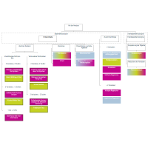
In the case of this example, the cluster analysis is conducted by means of a dataset containing the hypothetical data of 15 students. It includes the interval scaled variables of Period of use, Self-evaluation, Course attendance, and Age. Figure 1 shows how three clusters are formed based on the example data:
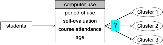
Figure 1: Example of the formation of three clusters
It is not yet possible to know how many clusters the students should be allocated to based on the variables being examined (it could be only two clusters, or more than three).
Figure 2 shows the values of two hypothetical variables in the form of a point cloud:
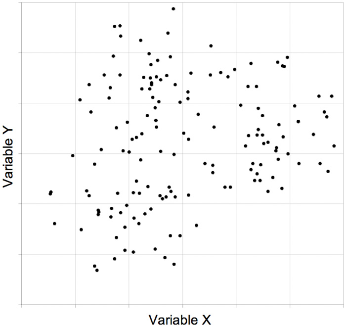
Figure 2: Point cloud
For two of the variables it is possible to depict the frame of reference visually. But as soon as three or more variables are involved, the data points can no longer be shown in two dimensions. Figure 3 shows three clusters that were formed by means of a certain cluster algorithm:
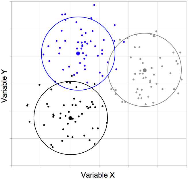
Figure 3: Point cloud with cluster formation
The criterion for forming the clusters in Figure 3 is the proximity among the respective points (units of analysis that are close to each other are allocated to the same cluster).
2.1 Determining the similarities
Conducting a cluster analysis means first calculating the proximity measurements with paired comparisons to determine how far apart two objects (in this case students) happen to be. There are two types of proximity measures: Similarity measures and distance measures. Similarity measures describe the similarity between two objects by comparing their content. Distance measures describe the similarity between two objects by measuring the geometric distance.
Table 1 provides an overview of the most important proximity measures that can be calculated:
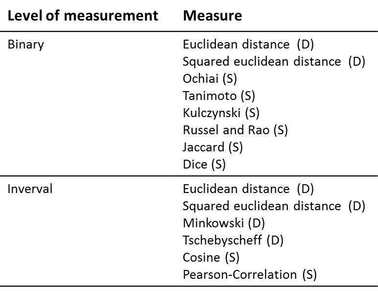
Table 1: Selected proximity measures Note: D = distance measure; S = similarity measure.
Nominal and/or ordinal scaled attributes are recoded into binary variables (with the dichotomous levels 0 or 1) before including them in the cluster analysis. A value of 1 will usually have a certain characteristic; in the case of a value of 0, this characteristic does not exist. A reduced number of categories as the result of dichotomization may cause a loss of information and lead to distortions. Distance measures rather than proximity measures are generally used for interval scaled variables. Here, SPSS calculates a distance matrix that compares all the objects with each other. Figure 4 shows a distance matrix of the example data:
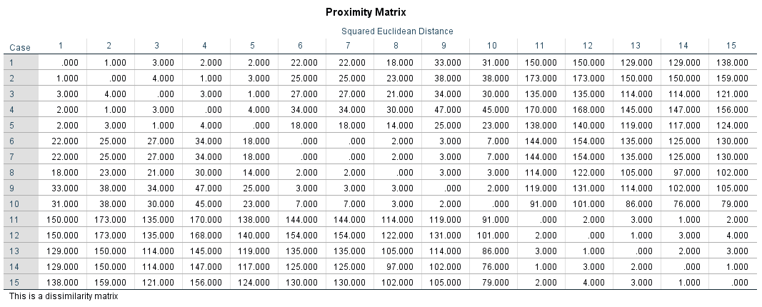
Figure 4: Distance matrix of the example data
The distance matrix is symmetrical: Every distance value is shown twice. The lower the values in Figure 4, the more similar the objects are.
2.2 Selecting the clustering algorithm
There are several options for forming clusters. Figure 5 shows a type of decision tree:
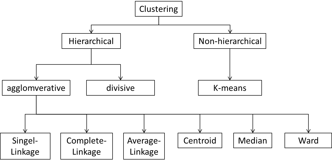
Figure 5: Cluster algorithms
This chapter focuses exclusively on the most frequently used hierarchical cluster analyses, which are subdivided into divisive and agglomerative methods.
In the case of divisive procedures, a large cluster is first formed from all the objects and then subdivided into smaller clusters. The agglomerative procedures, on the other hand, first examine the objects individually, which are then formed into clusters stepwise.
2.3 Determining the number of clusters
Although there are no generally valid criteria when it comes to determining the ideal number of clusters, content-related considerations often do play an important role. When choosing the number of clusters based on the data, the hierarchical cluster analysis (agglomerative procedure) can include a dendrogram, as shown in Figure 6 for the example data:
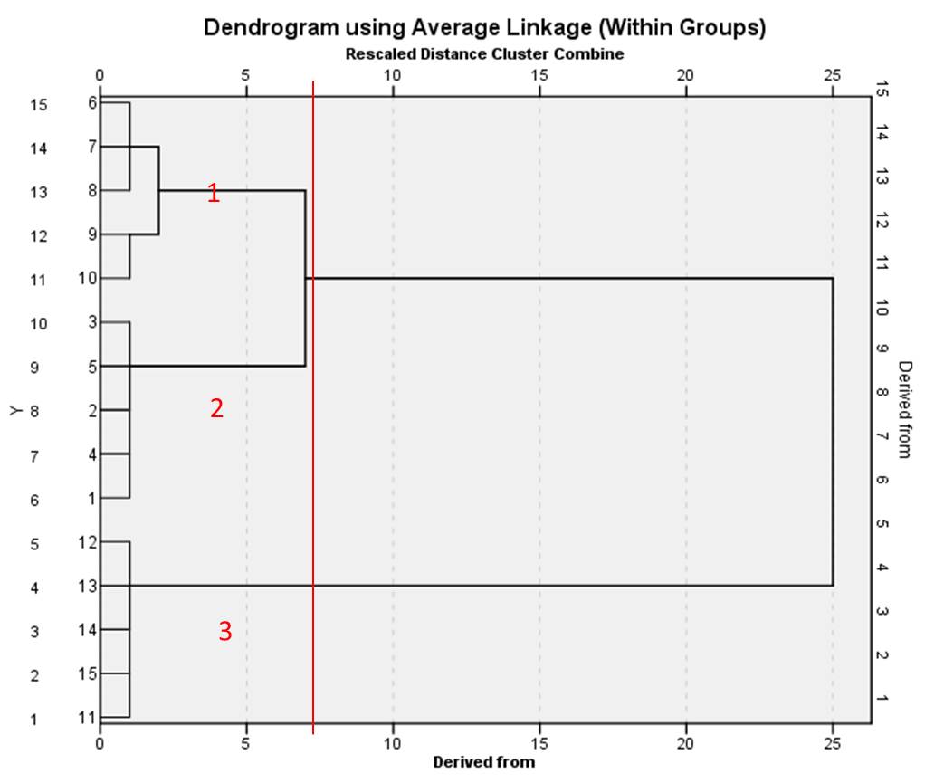
Figure 6: Dendrogram of the example data
The dendrogram visualizes all the steps of the cluster analysis as a graph, whereby the individual objects are depicted in the lines. The lines connecting the objects represent how the objects are merged into clusters. The heterogeneity values (shown in the columns) constitute transformed distances that are standardized on a scale of 0 to 25. A low value means that heterogeneity within the group is low. There is no generally valid cut-off value up to which the clusters should be selected. Clustering should be discontinued in every case if there are large gaps in heterogeneity. In the dendrogram of this example, the heterogeneity value jumps from 7 (see red line in Figure 6) to 25. It therefore makes sense to decide on the number of clusters that lie before a large jump: In the example, this would mean choosing three clusters (see red numbers in Figure 6).
Table 2 provides an overview of the clusters of the example data:
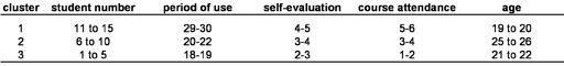
Table 2: Cluster overview of the example data. Note: “Period of use” = the period in hours; “Self-evaluation” = self-evaluation on a 5-point scale; “Course attendance” = number of IT courses attended
In this example, students allocated to Cluster 1 use computers more frequently than the average, rate their own skills as higher, have taken more IT courses, and are younger than the students allocated to Clusters 2 and 3. Forming clusters as in this hypothetical example enables the university to allocate students to groups so that the IT courses being offered can be tailored to their individual needs. The “Beginners” are allocated to Cluster 3, the “Advanced students” to Cluster 2, and the “Professionals” to Cluster 1.
3. SPSS commands
SPSS dataset: Example dataset used for the Clusteranalyse.sav
Click sequence: Analyze > Classify > Hierarchical clusters
Syntax:
CLUSTER period self course age
/METHOD WAVERAGE
/PRINT SCHEDULE
/PRINT DISTANCE
/PLOT DENDROGRAM VICICLE.
Distance matrix: In the “Statistics” window, select “Distance matrix”
Dendrogram: In the “Diagrams” window, select “Dendrogram”