1. Introduction
2. Procedure
3. Pearson chi-square distribution test with SPSS
4. SPSS commands
5. Literature
1. Introduction
The chi-square distribution test is a non-parametric statistical procedure with a chi-square-distributed test statistic that is used for comparing observed frequencies with expected frequencies. It tests, for example, if the observed distribution of the characteristics of a variable match with a theoretical distribution. The variables being tested can have any scale level.
2. Procedure
This chapter explains in detail the procedure of the chi-square distribution test based on the following question:
Does the frequency at which blood groups A, 0, B, and AB are found differ between a mountain village and Switzerland as a whole?
The procedure of the chi-square distribution test is summarized in three steps, which are described in the following section.
2.1 Determining the expected frequencies
The chi-square distribution test is used for comparing the observed frequencies with the expected frequencies. The default settings of SPSS are based on the assumption that all characteristics occur equally often. SPSS can be adjusted manually if the expected probability of the categories differs based on theoretical assumptions.
In this example, the chi-square distribution test is conducted with a dataset containing the blood types of 127 inhabitants of a hypothetical mountain village in Switzerland, whereby 52 inhabitants have blood type A, 44 have blood type O, 21 have blood type B, and 10 have blood type AB. The frequencies of blood types in all of Switzerland are known: 47% of the population has blood type A, 41% has blood type O, 8% has blood type B, and 4% has blood type AB. In a group of 127 persons, the expected absolute frequency at which blood type A occurs would therefore be 59.69, the expected absolute frequency at which blood type O occurs would be 52.07, the expected absolute frequency at which blood type B occurs would be 10.16, and the expected absolute frequency at which blood type AB occurs would be 5.08.
2.2 Calculating the test statistic
Calculating the test statistic of the chi-square distribution test involves comparing the observed frequencies and the expected frequencies as follows:
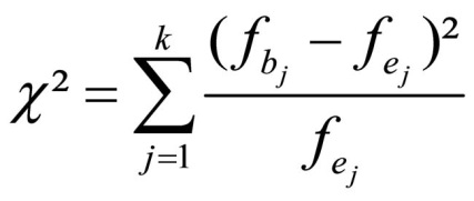
Figure 1: Calculating the chi-square test statistic
whereby
k = the number of attribute categories
fb = the observed absolute frequency in attribute category j
fe = the expected absolute frequency in attribute category j
If all attribute categories have an expected frequency of at least 5 units, the test statistic is close to being chi-square-distributed (degrees of freedom). In cases where the attribute categories have an expected frequency of less than 5 units, it makes sense to combine the neighboring categories based on factors relating to their content.
In this example, the expected frequencies of all attribute categories are greater than 5.
2.3 Testing for significance
This section explains how to determine the significance of the calculated test statistic. The calculated value is compared with the critical value of the chi-square distribution as determined by the degree of freedom.
In this example data, SPSS produces a chi-square test statistic of 18.572 and a p-value of .000 (see Chapter 3: “Chi-square distribution test with SPSS”). This value is less than .050, which means there are differences in the frequency at which the four blood types A, 0, B, and AB occur in the mountain village when compared to Switzerland as a whole.
3. Pearson chi-square distribution test with SPSS
SPSS produces the following figures when performing the chi-square distribution test:
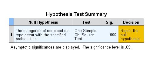
Figure 2: Summary of hypothesis testing
Figure 2 provides a summary of hypothesis testing using the example data. The null hypothesis stating that the observed distribution of the four blood types A, 0, B, and AB in a mountain village conforms with the expected distribution of Switzerland as a whole is rejected in favor of the alternative hypothesis.
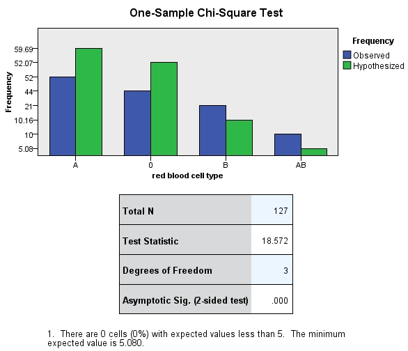
Figure 3: Cross table of the example data
Figure 3 shows the observed and the expected distributions (see under “Hypothesis”). It also shows the chi-square test statistic and the associated p-value. Because the calculated p-value is smaller than the significance level of .050, the observed distribution differs from the expected distribution. In the newer SPSS versions (from SPSS 19) it is possible to open the object in Figure 3 with a double-click on “Summary of hypothesis testing.”
4. SPSS commands
SPSS dataset: Example dataset used for the Chi-Quadrat-Verteilungstest.sav
Click sequence: Analysis > Nonparametric tests > One sample > Compare observed and hypothetical probabilities (chi-square test)
Define expected frequencies: Under “Options” > adjust “Expected probability”
Syntax: NPAR TESTS CHISQUARE
5. Literature
Field, A. (2009). Discovering statistics using SPSS. London: Sage Publications, Inc.
Gravetter, F. J. & Wallnau, L. B. (2009). Statistics for the behavioral sciences. Belmont: Wadsworth Cengage Learning.