1. Introduction
2. Procedure
3. Sign test with SPSS
4. SPSS commands
5. Literature
1. Introduction
The sign test is a non-parametric statistical procedure for determining whether there are differences in the central tendency of two dependent groups (paired samples). The test examines the same objects twice, whereby the measurements can take place at different times or involve two different forms of treatments (e.g. medications A and B). The dependent variable should be at least ordinal scaled. Because normal distribution is not a prerequisite, the sign test can be used in cases where the normal distribution prerequisite of interval scaled dependent variables is excessively violated and where carrying out a t-test for paired samples is not possible.
The sign test is a rank test in which the test statistic is calculated by forming differences in paired samples of dependent groups. The differences in paired samples are formed by allocating every value from the first group to the respective value from the second group. The two groups must have the same sample size. The disadvantage of the sign test is that, unlike in the case of the Wilcoxon Signed-Rank test, only the number of positive and negative differences in paired samples can be included in the calculation. The size of the differences in paired samples is not included.
2. Procedure
This chapter explains in detail the procedure of the sign test based on the following question:
Are there differences in the depression scores of patients before and six months after treatment begins?
The literature summarizes the procedure of the sign test in three steps, which are described in the following section.
2.1 Model formulation
The question is examined by means of a dataset with data of 24 patients suffering from depression. The answer to the question can be found with the help of a model, which in this case looks as follows:
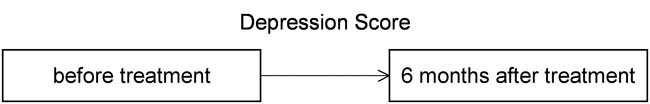
Figure 1: Example model
This example includes the interval scaled variables of “Depression scores” before treatment begins and six months after treatment begins.
2.2 Calculating the test statistic
This section explains how to calculate the test statistic. Table 1 shows the example dataset:
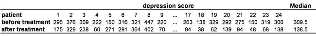
Table 1: Example data
The calculation of the test statistic is based on the differences in paired samples, which are shown in Table 2:
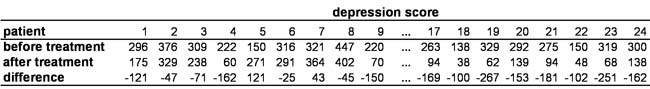
Table 2: Differences in paired samples
The calculation of the test statistic uses the differences in paired samples, which are unequal to zero. In this example, all 24 differences in paired samples are unequal to zero. The number of positive differences in paired samples is larger than the negative ones. If the central tendency at the two measurement times is the same, the number of positive and negative differences in paired samples will also be virtually the same, i.e. the probability of a positive difference in paired samples is 50%. The sign test determines significance by means of the binomial test, which determines whether the frequency distribution of one variable matches that of an assumed distribution.
The sign test uses the number of positive differences in paired samples as the test statistic (in the case of the example data, this value is 2).
2.3 Testing for significance
This section examines the significance of the test statistic by means of a binomial test. The separation value when using the sign test is always .500.
For this example, SPSS produces a p-value of .000 (see Chapter 3: “Sign test with SPSS”). Because this value is smaller than the significance level of .050, it can be assumed that the central tendency of the two measurement times differs significantly.
3. Sign test with SPSS
3.1 For older SPSS versions (up to SPSS 18) or the “Legacy Dialogs” in the newer versions
SPSS produces the following figures when performing the sign test:
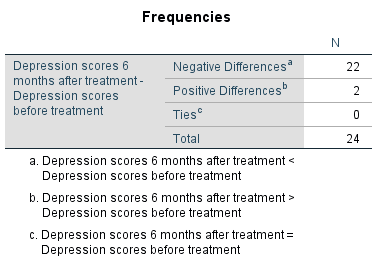
Figure 2: Number of differences in paired samples
Figure 2 shows the number of differences in paired samples of the two measurement times. “Ties” refers to the number of differences in paired samples that are equal to zero.
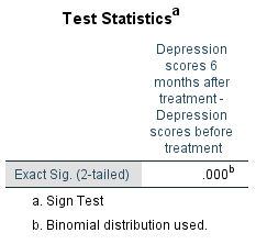
Figure 3: Number of differences in paired samples
Figure 3 shows the test statistic and the p-value, which is smaller than the significance level of .050. It can therefore be assumed that the “Depression scores” of patients are significantly smaller six months after treatment began than they were before.
3.2 For newer SPSS versions (from SPSS 19)
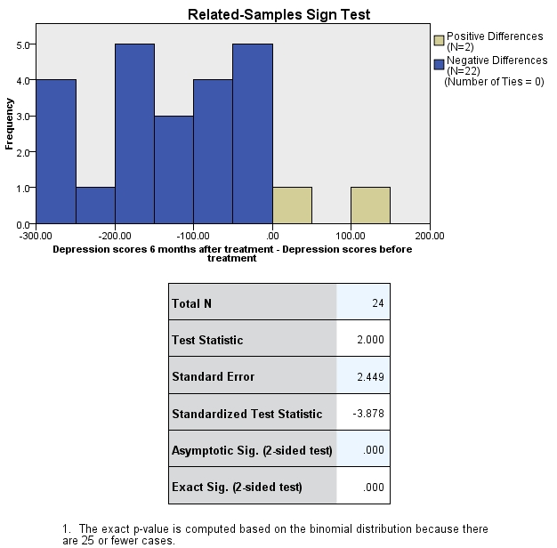
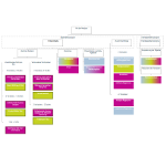
Figure 4: Model viewer
Figure 4 shows the “Model viewer” of the sign test, which in the newer SPSS versions can be opened with a double-click on “Summary of hypothesis testing.”
4. SPSS commands
SPSS dataset: Example dataset used for the Vorzeichentest.sav
Click sequence: Analyze > Non-parametric tests > Two paired samples
In the “Test pairs” field > Define dependent groups (“Samples”)
Syntax: NPAR TESTS SIGN
5. Literature
Gravetter, F. J. & Wallnau, L. B. (2012). Statistics for the behavioral sciences. Belmont: Wadsworth Cengage Learning.