1. Introduction
2. Procedure
3. Multivariate analysis of variance with SPSS
4. SPSS commands
5. Literature
1. Introduction
Analyses of variance (ANOVA) are among the most frequently used statistical procedures, especially in the social sciences. There are several types of analyses of variance that differ in the number of independent variables and based on whether there are any repeated measures. This chapter focuses on the multivariate analysis of variance, which examines the influence of several independent variables as well as their interaction effect on one dependent variable. The independent variables (also referred to as “factors”) are generally nominal scaled or ordinal scaled. The dependent variable should be interval scaled and close to normal distributed.
2. Procedure
This chapter explains in detail the procedure of the one-way repeated measures analysis of variance based on the following question:
Do education levels and gender influence the annual income of US citizens? Is there an interaction effect between education levels and gender on the annual income of US citizens?
The multivariate analysis of variance is summarized in five steps, which are described in the following section.
2.1 Schematic representation
The question is examined based on data from the US Bureau of Labor Statistics” in March 2002, whereby the analysis relies on a subsample (n = 1503 adult US citizens). The answer to the questions can be found with the help of a schematic representation, which in this case looks as follows:
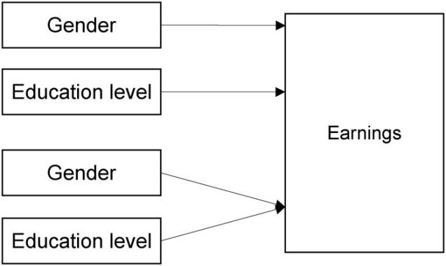
Figure 1: Schematic representation
The schematic representation indicates that gender and education levels each have a separate effect on annual income. In addition, there could be some form of interaction between education levels and gender.
The independent, ordinal scaled “education levels” variable has six levels (1 = “no high school”, 2 = “some high school”, 3 = “high school diploma”, 4 = “some college”, 5 = “Bachelor’s degree” and 6 = “postgraduate degree”). The dependent “annual income” variable (in US dollars) is interval scaled.
2.2 Calculating the test statistic
Figure 2 shows the descriptive statistics of the example data (separated by the independent “gender” and “education levels” variables):
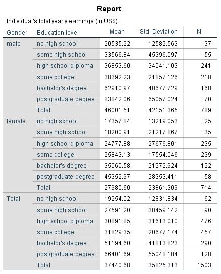
Figure 2: Descriptive statistics of the example data. Note: M = mean; SD = standard deviation
SPSS can display the means as a diagram, which can be produced via the “Diagrams” option in the “Univariate” dialogue box and by selecting the respective variables under “Horizontal axis.”
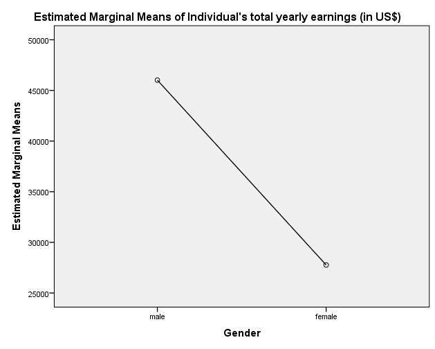
Figure 3: Graphic representation of the means for the independent “Gender” variable.
Figure 3 shows that the means of the annual income (in US dollars) vary between men and women. The analysis of variance makes it possible to determine whether these differences in the means are statistically significant once the associated test statistic has been calculated.
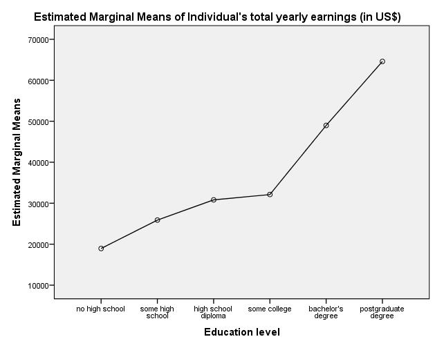
Figure 4: Graphic representation of the means of the independent “education levels” variable.
Figure 4 shows that the means of the annual income (in US dollars) vary between the different education levels. The analysis of variance makes it possible to determine whether these differences in the means are statistically significant once the associated test statistic has been calculated.
In addition, the multivariate analysis of variance can be used for determining whether significant interaction effects exist among the independent variables, i.e. if the interaction effect of the independent variables has a significant influence on the dependent variable. The following figure depicts the interaction effect graphically:
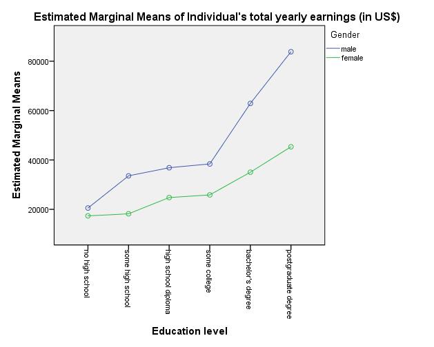
Figure 5: Graphic representation of the interaction effect
Figure 5 shows that the lines of the genders are not parallel, indicating that an interaction effect exists. Once the associated test statistic has been calculated, the multivariate analysis of variance can be used for determining whether the interaction effect is significant.
The underlying idea of the analysis of variance is based on the decomposition of the entire variance of the dependent variables. The total variance is separated into the variance within groups and the variance between groups. The variance between groups in turn is separated into the variances that are influenced by the factors and the variances that are influenced by the interactions.
In the case of a multivariate analysis of variance with two independent variables, the total variance is calculated as follows:
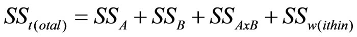
Figure 6: Calculating the total variance
whereby
SS = the sum of squared differences
A = the first factor (independent variable)
B = the second factor (independent variable)
AxB = the interaction of the two factors (independent variables)
The total variance can also be described with the following equation:
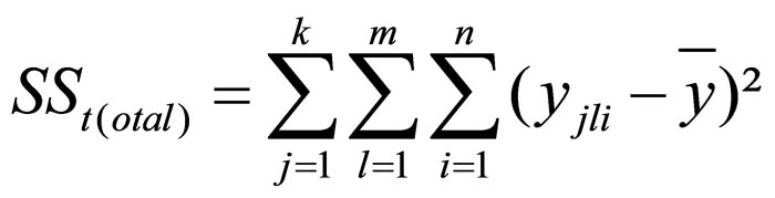
Figure 7: Equation of the total variance (complete equation)
whereby
SS = the sum of squared differences
k = the number of factor levels of factor A
j = the factor level of factor A
m = the number of factor levels of factor B
l = the factor level of factor B
n = the sample size
y = the total mean
yjli = the attributes of unit of analysis i in factor levels j and l
If more than two factors (independent variables) are involved, the equation is extended accordingly.
The influence of the first factor is calculated as follows:
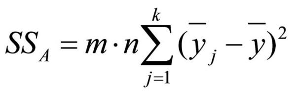
Figure 8: Equation of the variance of the first factor
whereby
SS = the sum of squared differences
m = the number of factor levels of factor B
n = the sample size
k = the number of factor levels of factor A
j = the factor levels of factor A
yj = the mean of factor level j of factor A
y = the total mean
The influence of the second factor is calculated as follows:
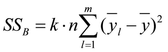
Figure 9: Equation of the variance of the second factor
whereby
SS = the sum of squared differences
k = the number of factor levels of factor A
n = the sample size
m = the number of factor levels of factor B
l = the factor levels of factor B
yj = the mean of factor level l of factor B
y = the total mean
The variance that arises through the interaction effect of the two variables is calculated as follows:
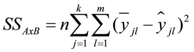
Figure 10: Equation of the variance of the interaction effects
whereby
SS = the sum of squared differences
n = the sample size
k = the number of factor levels of factor A
j = the factor levels of factor A
m = the number of factor levels of factor B
l = the factor levels of factor B
yjl = the mean of factor levels j and l
ŷjl = the estimated value (without interaction) for the mean of factor levels j and l
The estimated value is the common mean that can be expected based on the assumption that there is no interaction between the two factors and is calculated as follows:
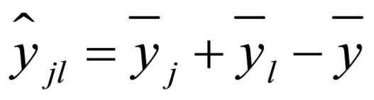
Figure 11: Calculating the estimated value
whereby
ŷjl = the estimated value (without interaction) for the mean of factor levels j and l
yj = the mean of factor level j of factor A
yj = the mean of factor level l of factor B
y = the total mean
The following equation describes the sum of squared differences of the individual values from the respective group mean (“within” the groups):
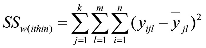
Figure 12: Equation of the variance within the groups
whereby
SS = the sum of squared differences
k = the number of factor levels of factor A
j = the factor levels of factor A
m = the number of factor levels of factor B
l = the factor levels of factor B
n = the sample size
yjli = the attributes of unit of analysis i in factor levels j and l
yjl = the mean of factor levels j and l
The following table shows the degrees of freedom with which the individual variances are standardized to obtain the respective variances:

Table 1: Degrees of freedom
The test statistics of the main effects and the interaction effect are calculated by dividing the calculated variances by the variance within the groups:
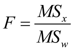
Figure 13: Calculating the test statistic
The F-distributed test statistics is compared with the critical value of the theoretical F-distribution as determined by degrees of freedom.
2.3 Testing for homogeneity of variance
Homogeneity of variance between the groups is a prerequisite for conducting a multivariate analysis of variance.
Before calculating the analysis of variance, it is therefore necessary to test for homogeneity of variance. This means using the Levene test, which is an extension of the F-test. In SPSS, the test for homogeneity of variance can be selected in the “Univariate” dialogue box of the “Options” menu. For the Levene test, the null hypothesis states that the variances of the different groups are homogeneous.
In the case of the example data, SPSS produces a p-value of .000 for the Levene test when determining homogeneity of variance (see Chapter 3: “Multivariate analysis of variance with SPSS”). The literature explains that the p-value of the test for homogeneity of variance should be greater than .100 if heterogeneous variances are to be excluded. The p-value of the example data indicates that the variances are not homogeneous and that the prerequisite of homogeneity of variance is therefore not met.
Because the example data involves a large sample (n = 1503), the multivariate analysis of variance can be carried out even if the prerequisite of homogeneity of variance is violated.
2.4 Testing for significance
This section explains how to determine the significance of the calculated test statistic. The F-value is compared with the critical value of the theoretical F-distribution.
In his example, the two main effects and the interaction effect are calculated.
For the example data, SPSS produces a test statistic F of 64.923 for the “Gender” variable and a p-value of .000, and a test statistic F of 37.539 and a p-value of .000 for the “education level” variable (see Chapter 3: “Multivariate analysis of variance with SPSS”). These values are below the significance level of .050. The null hypotheses of the main effects can be rejected in favor of the alternative hypotheses. Both independent variables have an influence on the dependent variable. Consequently there are significant differences in the annual income of men and women as well as between at least two categories of the “education level” variable. Because in the case of independent variables with more than two gradations the multivariate analysis of variance tests only for one difference, post hoc tests can be conducted afterwards to determine which means of the various categories differ significantly from the others.
For the interaction between gender and education level, SPSS shows a test statistic F of 5.926 and a p-value of .000 (see Chapter 3: “Multivariate analysis of variance with SPSS”). This value is smaller than the significance level of .050. The interaction of both independent variables influences the dependent variable. The graphic representation of the interaction effect (see Figure 5) indicates that the two independent variables influence each other. With a rising “education level,” the difference in the means of annual income between men and women rises as well. For lower “education level,” there are virtually no differences in the means of the annual income; however, for high “education level” men earn significantly more.
2.5 Post hoc tests
In the case of independent variables with more than two levels, the multivariate analysis of variance provides no information about which group means differ significantly from the others. For this, post hoc tests with paired comparisons of groups can be carried out to determine which differences in the means have caused the analysis of variance to produce a significant result. With respect to the post hoc tests, it is worthwhile to consider the “conservative” Scheffé Test, because this would lower the chance of any randomly arising correlations becoming significant.
The probability of committing a Type 1 error (the erroneous assumption of an alternative hypothesis) increases with the number of tests carried out. To remedy this problem, the significance level is corrected by the number of tests that are carried out. SPSS has several options for making this adjustment, which can be selected under “Post Hoc” in the “Univariate” dialogue box. It is worthwhile to compare the results of the different procedures.
3. Multivariate analysis of variance with SPSS
When carrying out the multivariate analysis of variance, SPSS produces the following figures, among other things:
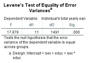
Figure 14: Levene test for homogeneity of variance
Figure 14 shows the results of the Levene test for homogeneity of variance. A significant result indicates that the variances of the individual groups differ and that the prerequisite of the analysis of variance is not met. In this example, the p-value is .000, which indicates that the variances are not homogeneous. Despite the large sample size, it is nevertheless possible to do further calculations.
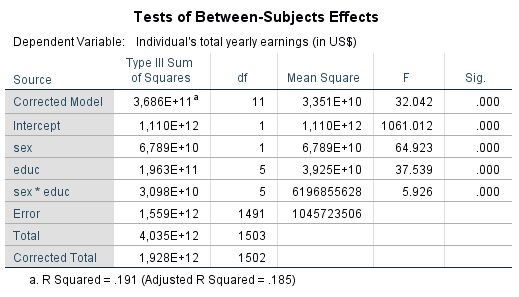
Figure 15: Test statistic of multivariate analysis of variance
Figure 15 shows the result of the multivariate analysis of variance. The two main effects (gender, educ.) and one interaction effect (gender * educ.) were examined.
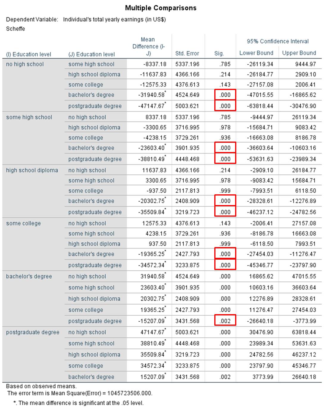
Figure 16: Test statistic of multivariate analysis of variance
In Figure 16, the second column shows the differences between the respective groups, whereby the p-values in the fourth column are relevant. There are significant differences between certain groups. For example, there is a significant difference in annual income (see red marking in Figure 16) between individuals without a high school diploma and those with a Bachelor’s or university degree. Because the p-values derived from these comparisons are less than .050, it can be assumed that these means differ significantly.
4. SPSS commands
SPSS dataset: Example dataset used for the Mehrfaktorielle-Varianzanalyse.sav
Click sequence: Analysieren > allgemeines lineares Modell > Univariat
Syntax:
UNIANOVA earn BY sex educ
/METHOD=SSTYPE(3)
/INTERCEPT=INCLUDE
/POSTHOC=educ(SCHEFFE)
/PLOT=PROFILE(sex educ educ*sex)
/EMMEANS=TABLES(sex) COMPARE ADJ(BONFERRONI)
/EMMEANS=TABLES(educ) COMPARE ADJ(BONFERRONI)
/PRINT=HOMOGENEITY DESCRIPTIVE
/CRITERIA=ALPHA(.05)
/DESIGN=sex educ sex*educ.