1. Introduction
2. Procedure
3. T-test with SPSS
4. SPSS
5. Literature
1. Introduction
The t-test for two independent samples can be used to determine whether there is a statistically significant difference between the means of two independent samples. The t-test is thus suitable for verifying a difference hypothesis between two independent samples. The variable to be tested should therefore be interval scaled (LINK to scale level) and normal distributed. Unlike in the case of the t-test for paired samples, the samples do not need to be of the same size.
1.1. Possible problem formulations
The t-test for two independent samples is used for answering the question of whether two groups differ in terms of a certain characteristic (consumer behavior, social inclusion, stress-resistance, attitude towards factual issues, etc.) or if an experimental group produces results that vary from those of a control group (success in treatment, effects of certain tests, etc.). This t-test therefore is suitable for questions such as “Does the consumer behavior of men and women differ?” or “Does the experimental group and the control group respond differently to a treatment method?”.
2. Procedure
2.1 Hypothesis formulation
The procedure for conducting a t-test for two independent samples is explained based on a question taken from marketing research.
A group of respondents consisting of roughly half men and half women is asked to rate the quality of a product on a scale of 0 to 10, whereby 0 = “very bad” and 10 = “very good.” The research question can be formulated as follows: Do women and men rate the quality of the product differently?
The aim of the research is to find out if a product’s quality appeals equally to men and women.
2.1 Hypothesis formulation
To test the research question statistically, it is necessary to formulate hypotheses. It should thus be possible to find out if the difference in the sample means can be generalized onto the population underlying the samples.
The null hypothesis and the alternative hypothesis are as follows:
H0: μ1=μ2 The means of the two parent populations are the same.
HA: μ1≠μ2
The means of the two parent populations differ.
2.2 Calculating the test statistic
To test the hypothesis, it is first necessary to obtain data (see Table 1: Example data).
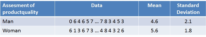
Table 1: Example data
Based on the means from “Table 1: Example data,” it can be assumed that women and men rate product quality differently. With the help of the t-test it is now possible to determine if this difference is also statistically significant.
The name of the test is derived from the test statistic, which is t-distributed if the null hypothesis proves to be valid. The test statistic t can be shown as follows:
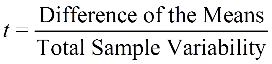
Numerators and denominators are calculated as follows:
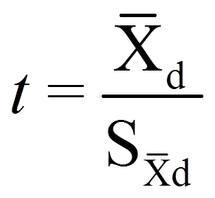
Sx – x = the standard deviation of the difference of the means
Xk = the mean of the xk variable
Note: The test value for a t-test with two independent samples is t-distributed with degrees of freedom (n1 + n2 – 2).
The calculated test statistic must then be compared with the critical value, which is determined by the number of degrees of freedom.
2.3 Conducting the hypothesis test
A further prerequisite for the t-test for two independent samples is the homogeneity of the variances of both samples (s21≈s22). When comparing the test statistic with the critical value it is therefore important to note whether the variances of the two samples are the same and if homogeneity of variance is thus given.
- Testing for homogeneity of variance: The condition of homogeneity of variance can be determined with the help of the Levene test, which is an extension of a simple F-test (LINK to F-test). If the prerequisite of homogeneity of variance is violated, the degrees of freedom of the test statistic will need to be adjusted. Note: Compared to the F-test, the Levene test is more robust when it comes to determining violations of the normal distribution assumption.
- Testing for significance: After the test for homogeneity of variance, the calculated test statistic can be tested for significance. The calculated t-value is therefore compared with the critical value of the test statistic.
3. T-test with SPSS
The following figures show the results of the t-test in he sequence as produced by SPSS. From Figure 1: Group statistics indicate the size of the sample, the mean, and the standard deviation of the sample.
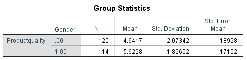
Figure 1: Group statistics
Test for homogeneity of variance:
The test for homogeneity of variance aims to support the null hypothesis, i.e. the F-value should not become significant. For this example, SPSS produces an F-value of 1.864 and an associated significance (p-value) of .173 (see Figure 2: Test for homogeneity of variance). The significance of .173 in the result is greater than the significance level of α =.050 and thus supports the assumption that homogeneity of variance is given.
Figure 2: Testing for homogeneity of variance
Testing for significance:
For this example, SPSS produces a t-value of -3.834 (see Figure 3: Test statistic). This value still needs to be tested for significance. Since it has been determined that homogeneity of variance is given, the significance level in SPSS must be taken from the “Equal variances assumed” row. This example shows a significance (p-value) of .000, which is smaller than the significance level of .050. It can therefore be assumed that the means differ with respect to gender.
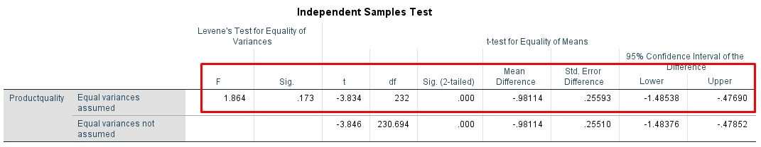
Figure 3: Testing for significance
Note: Whether the null hypothesis can be rejected depends on the variance and size of the sample n, among other things. A large sample may result in a test producing a significant result more quickly. If the test statistic is significant, the question arises as to whether the results are also of practical relevance. Here, the measure of the effect size is useful because it makes it possible to draw conclusions about the practical relevance of a significant test result and because it is virtually unaffected by sample size n.
Cohen’s d (Cohen 1992) has become the established way of measuring effect size. It is not possible to calculate Cohen’s d with SPSS. However, it can be calculated with the G*Power (LINK to the program) program.
4. SPSS
Click sequence: Analyze > Compare means > Independent samples t-test
Note: The grouping variable serves to allocate the respective sample.
Syntax: T-TEST GROUPS
5. Literature
Field, Andy (2009). Discovering Statistics Using SPSS. 316-346.
Cohen, Jacob (1992). A power primer. Psychological Bulletin, 112: 155-159.