1. Introduction
2. Procedure
3. Friedman test with SPSS
4. SPSS commands
5. Literature
1. Introduction
The Friedman test is a non-parametric statistical procedure used for determining whether there are differences in the central tendency of more than two dependent groups (or samples). The test examines the same objects repeatedly, for example by measuring different times or multiple treatments (e.g. medications A, B, or C). The dependent data are ranked within each unit of analysis (e.g. test person), and the groups must be of the same sample size. The dependent variable should be at least ordinal scaled. The Friedman test can be used in cases where the normal distribution prerequisite of interval scaled dependent variables is excessively violated and where carrying out a one-way analysis of variance with repeated measures is not possible.
The Friedman test (also referred to as analysis of variance by ranks) is a rank test in which the test statistic is calculated by comparing multiple ranking sequences. The underlying idea is that the data of the dependent groups in a sequence of joint ranks will have the same distribution if it has the same central tendency. The Friedman test is an extension of the Wilcoxon Signed-Rank test for two dependent groups.
2. Procedure
This chapter explains in detail the procedure of the Friedman test based on the following question:
Are there differences in the severity of acne among patients at different measurement times (before the treatment, and 4, 8, and 12 weeks after the treatment began)?
The literature summarizes the Friedman test in four steps, which are described in the following section.
2.1 Model formulation
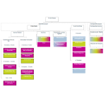
The question is examined based on a dataset from the University of York. The data is on 14 patients with acne who received medication over a 12-week period. During this time, changes in the severity of the acne was measured on a 12-point scale. The answer to the question can be found with the help of a model, which in this case looks as follows:
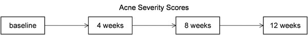
Figure 1: Example model
This example considers the 12-level dependent variables of “Acne Severity Scores” before the treatment starts and 4, 8, and 12 weeks after the start date.
2.2 Calculating the test statistic
This section explains how to calculate the test statistic. Table 1 shows the example data as well as the calculation of the sums of ranks of the different measurement times:
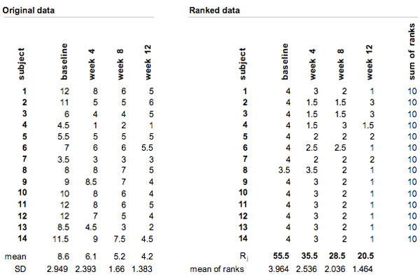
Table 1: Example data with calculations of the sums of ranks
The values of the Acne Severity Score are ranked within every test person. In the case of ties (same value for multiple measurement times), the averages of the rank are calculated. Four weeks and eight weeks after the beginning of the treatment, the third test person, for example, had an “Acne Severity Score” of 4, which corresponds to the first and the second rank within the person. Here, the rank value of 1.5 (mean of the two ranking positions) is assigned twice. The sums of ranks of the measurement times are formed by adding up all the ranking positions.
The test statistic FR of the Friedman tests is calculated as follows:
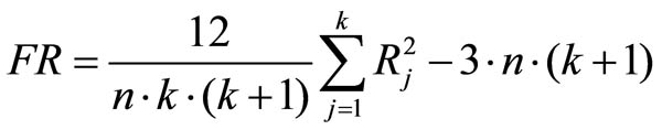
Figure 2: Calculating the test statistic H
whereby
n = the sample size (the same for every measurement time)
j = the measurement time j
k = the number of measurement times
Rj = the sum of ranks at measurement time j
SPSS automatically calculates the sums of ranks of all measurement times as well as the test statistic FR of the Friedman test.
2.3 Testing for significance
This section examines the test statistic for significance. If the sample size for three measurement times is larger than 10 and/or for more than three measurement times larger than 5 (as in this example), the test statistic FR has a Chi² distribution. In this case, the calculated FR value is compared with the critical value of the Chi² distribution as determined by the degrees of freedom. SPSS performs the comparison automatically.
The working hypothesis of the Friedman test states that the ranking positions of the different measurement times are evenly aligned in the sequence of joint ranks. In this example, SPSS produces a p-value of .000 (see Chapter 3: “Friedman test with SPSS”). Because this value is smaller than the significance level of .050, it can be assumed that the ranking positions of the different measurement times in the sequence of joint ranks are not distributed evenly.
2.4 Post hoc tests
The Friedman test provides no information about which medians or median differ(s) significantly from the others. For this, post hoc tests (in this case “manually” through the Wilcoxon Signed-Rank test) that examine paired comparisons of the groups can be carried out to determine which differences in the central tendencies caused the Friedman test to produce a significant result. The new SPSS version can perform post hoc tests automatically: A double-click on “Summary of hypothesis testing” will open the “Model viewer,” in which “Paired comparisons” can be selected from “Display” (see Chapter 3: “Friedman test with SPSS”).
3. Friedman test with SPSS
3.1 For older SPSS versions (up to SPSS 18) or the “Legacy Dialogs” in the newer versions
SPSS produces the following figures when performing the Friedman test:
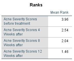
Figure 3: Mean ranks
Figure 3 shows the mean ranks of the “Acne Severity Scores” of the individual measurement times of the example data. The mean rank of the “Acne Severity Scores” is largest before the treatment begins and smallest 12 weeks after the treatment begins.
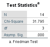
Figure 4: Test statistic
Figure 4 shows the test statistic and the p-value, which is smaller than the significance level of .050. It can therefore be assumed that at least one of the mean ranks differs significantly from the others.
3.2 For newer SPSS versions (from SPSS 19)
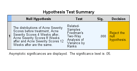
Figure 5: Summary of hypothesis testing
Figure 5 summarizes hypothesis testing. The null hypothesis according to which the ranking positions of the different measurement times are distributed evenly in the sequence of joint ranks is rejected in favor of the alternative hypothesis.
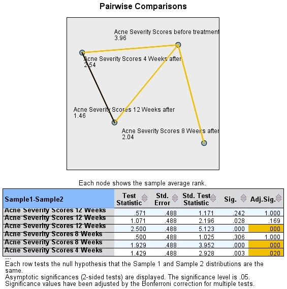
Figure 6: Post hoc tests
Figure 6 shows the paired comparisons of the measurement times. The post hoc tests indicate that the mean rank of the “Acne Severity Scores” before the treatment begins differs significantly from the mean ranks as measured 4, 8, and 12 weeks after the treatment begins. There are no significant differences in the mean ranks of the “Acne Severity Scores” between 4, 8, and 12 weeks after the beginning of the treatment.
4. SPSS commands
SPSS dataset: Example dataset used for the Friedman-Test.sav
Click sequence: Analyze > Nonparametric Tests > Legacy Dialogs > k Related Samples…
Syntax: NPAR TESTS FRIEDMAN
5. Literature
Field, A. (2009). Discovering Statistics Using SPSS. London: Sage.
Gravetter, F. J. & Wallnau, L. B. (2009). Statistics for the behavioral sciences. Belmont: Wadsworth Cengage Learning.