
1. Introduction
2. Procedure
3. Levene test with SPSS
4. SPSS commands
5. Literature
1. Introduction
The F-test is a statistical procedure in which the test statistic is F-distributed. The F-test can be used for determining whether the variances of two samples (or groups) differ from each other. The dependent variable should be at least ordinal scaled and normal distributed.
The F-test and its associated procedures are used, for example, for determining whether variance analyses meet the prerequisite of homogeneity of variance.
2. Procedure
This chapter explains in detail the F-test procedure based on the following question:
Does the variance in internet usage (in hours per week) differ between women and men?
The F-test is summarized in three steps, which are described in the following section.
2.1 Model formulation
The question is examined by means of a randomly generated subsample (n = 652 adult US citizens) of the General Social Survey (GSS) of the year 2000.
The answer to the question can be found with the help of a model, which in this case looks as follows:
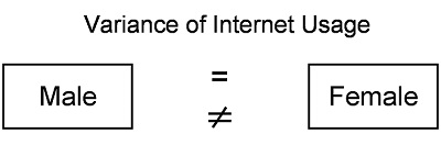
Figure 1: Example model
In this example, the dependent variable of “Internet usage” (hours per week) is separated based on gender.
2.2 Calculating the test statistic
The example dataset includes 305 men and 347 women. Table 1 shows the means and standard deviations of the dependent “Internet usage” variable for both genders:
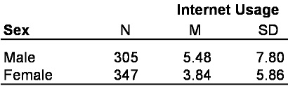
Table 1: Example data Note: N = sample size; M = mean; SD = standard deviation
The standard deviation of the dependent variable “Internet usage” is 7.80 for men and 5.86 for women. The F-test determines if the difference of the variances is significant. The variance equals the square of the standard deviation.
In this case, the test statistic is the F-statistic with the theoretical F-distributions and the associated degrees of freedom that are used for determining whether the difference of the variances is significant.
The test statistic of the F-test is calculated as follows:
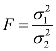
Figure 2: Calculating the F-value
whereby
σ1² = the variance of the first sample
σ1² = the variance of the second sample
The value of F is 1 if the variances of the two samples are identical, and it is either greater or less than 1 in cases where the variances of the two samples differ.
It is not possible to conduct the F-test with SPSS directly. When conducting a one-way analysis of variance, the Levene test can be used as an alternative to the “classical” F-test by selecting “Homogeneity of variance test” in the “Options” dialogue box. The Levene test is more robust if the normal distribution of dependent variables is violated, and it also can be used when more than two samples are involved.
The following section explains how to conduct the F-test manually (see Chapter 3: “Levene with SPSS” for a computer-assisted calculation). In this example, the F-value is calculated as follows:
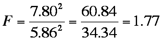
Figure 3: Calculating the F-value in this example
The F-value is subsequently compared with the critical value of the theoretical F-distribution as given by the degrees of freedom.
2.3 Testing for significance
This section explains how to determine the significance of the calculated test statistic. When comparing the calculated F-value with the critical value, the numerator degrees of freedom and the denominator degrees of freedom that are obtained by reducing the sample size by one (nx – 1) are relevant. The critical values are shown in the F-tables.
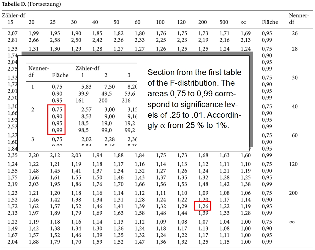
Table 2: Extract from an F-table (Bortz & Schuster, 2010)
In this example, the numerator degree of freedom is 346 (347-1) and the denominator degree of freedom is 304 (305-1). Because these degrees of freedom do not appear in the table, the critical value is taken from the nearest column or row, which is defined through smaller degrees of freedom (in this case: df1= 200 and df2= 200). The F-table shows the critical value of the significance levels .25, .10, .50 and .01 in descending order. In this example, a significance level of .05 is selected, whereby the relevant critical value is 1.26 (see red marking in Table 2). The calculated test statistic is greater than the critical value (1.77 > 1.26). It can therefore be assumed that the differences in the variances of the “Internet usage” variable assigned to both genders are significant.
3. Levene test with SPSS
SPSS produces the following figure when conducting the one-way analysis of variance (select “Homogeneity of variance test” under “Options”):
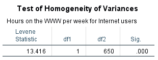
Figure 4: Levene test for homogeneity of variance
Figure 4 shows the Levene test. Because the output p-value is less than .050, it can be assumed that the variances of the “Internet usage” variable assigned to both genders differs significantly. The variance of internet usage (hours per week) among men is significantly greater than in women. The corresponding dataset also indicates that there are differences in the means of internet usage between genders (no further explanation of their calculation is shown at this point). It can thus be concluded that men spend significantly more hours per week on the internet than women.
4. SPSS commands
SPSS dataset: Example dataset used for the F-Test.sav
Click sequence: Analysis > Compare means > One-way analysis of variance (ANOVA)
Under “Options” select “Homogeneity of variance test”
Syntax:
ONEWAY AV BY UV
/STATISTICS HOMOGENEITY
/MISSING ANALYSIS.
5. Literature
Field, A. (2009). Discovering Statistics Using SPSS. London: Sage.
Bortz, J. & Schuster, C. (2010). Statistik für Human- und Sozialwissenschaftler. Berlin: Springer.