1. Introduction
2. Procedure
3. One-way repeated measures analysis of variance with SPSS
4. SPSS commands
5. Literature
1. Introduction
Analyses of variance (ANOVA) are among the most frequently used statistical procedures, especially in the social sciences. There are several types of analyses of variance that differ in the number of independent variables and based on whether there are any repeated measures. This chapter focuses on the one-way repeated measures analysis of variance, which examines differences in the means of three or more different groups (or samples) at different measurement times. The test examines the same objects repeatedly, for example by measuring different times or multiple treatments (e.g. medications A, B, or C). The dependent variable should be interval scaled and close to normal distributed. The independent variable is usually nominal scaled and referred to as “factor.”
2. Procedure
This chapter explains in detail the procedure of the one-way repeated measures analysis of variance based on the following question:
Are there differences among husbands in the values of the “Desire to express worry” scale at different measurement times (right after the wedding and after 5, 10 and 15 years of marriage)?
The literature summarizes the one-way repeated measures analysis of variance in five steps, which are described in the following section.
2.1 Schematic representation
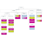
The question is examined based on a dataset from the University of Canberra. The data is on 30 husbands who have completed the “Desire to Express Worry” questionnaire at different measurement times. The inquiry aims to find out if the length of the marriage could influence the extent to which men are willing to share their worries with their wife. The answer to the question can be found with the help of a schematic representation, which in this case looks as follows:
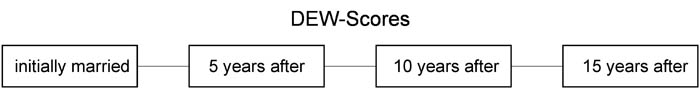
Figure 1: Schematic representation Note: DEW = desire to express worry
The schematic representation states that the means of the “Desire to Express Worry” scale can differ at the different measurement times (1 = right after the wedding, 2 = five years after the wedding, 3 = ten years after the wedding, and 4 = fifteen years after the wedding). In general, the null hypothesis of the analysis of variance with repeated measures is as follows:
Figure 2: Null hypothesis of analysis of variance with repeated measures with four measurement times
The alternative hypothesis states that the null hypothesis is not valid, i.e. that there are differences in the mean.
2.2 Calculating the test statistic
The sample dataset includes 30 test subjects (in this case husbands) who were examined at four measurement times. Table 1 shows the raw data as well as the means and standard deviations (separated by measurement times):
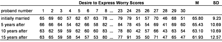
Table 1: Example data Note: M = mean; SD = standard deviation
Chapter 3 (“One-way repeated measures analysis of variance with SPSS”) explains how to determine a factor in SPSS.
SPSS can display the means as a diagram, which can be produced by selecting “Diagrams” from the dialogue box of the one-way analysis of variance (ANOVA) with repeated measure (“Factor 1” is added under “Horizontal axis”).
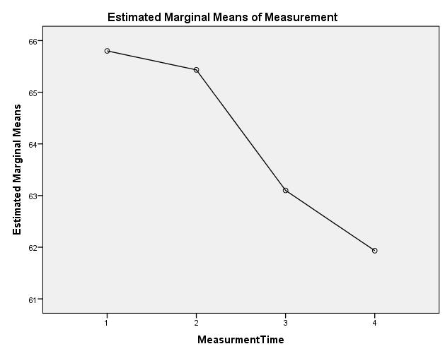
Figure 3: Graphic representation of the means Note: 1 = right after the wedding, 2 = five years after the wedding, 3 = ten years after the wedding, and 4 = fifteen years after the wedding
As shown in Figure 3, the means of the “Desire to Express Worry” scale differ at the various measurement times. The one-way repeated measures analysis of variance makes it possible to determine whether these differences in the means are statistically significant once the associated test statistic has been calculated.
The underlying idea of the analysis of variance with repeated measures or without repeated measures is the same and is based on a decomposition of the total sample variance of the dependent variables. Because the groups consist of the same objects, the variance between the groups is irrelevant for the analysis of variance with repeated measures. The total variance is calculated by adding up the variance between groups:
Figure 4: Calculating the total variance
whereby
SS = the sum of squared differences
zw = between groups
in = within groups
The total variance can also be described with the following equation:
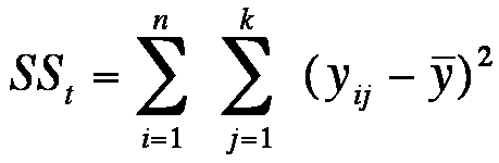
Figure 5: Total variance (complete equation)
whereby
SS = the sum of squared differences
j = the factor level
k = the number of factor levels
n = the sample size
y = the total mean
yij = the attributes of unit of analysis i in factor level j
SSzw describes the differences between groups and is calculated as follows:
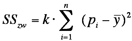
Figure 6: Equation of the variance between groups
whereby
SS = the sum of squared differences
k = the number of factor levels
n = the sample size within a factor level
pi = the mean of all the measured values of unit of analysis i
y = the total mean
SSin describes the differences of one unit of analysis between the different measurement times and is calculated as follows:
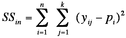
Figure 7: Equation of the variance within groups
whereby
SS = the sum of squared differences
j = the factor level
k = the number of factor levels
n = the sample size within a factor level
pi = the mean of all the measured values of unit of analysis i
yij = the attributes of unit of analysis i in factor level j
SSin can also be separated into the treatment variance and residual variance:
Figure 8: Equation of the decomposition of the variance within groups
- Figure 8: Equation of the decomposition of the variance within groups
The treatment variance describes the differences of the groups between the various measurement times and is calculated as follows:
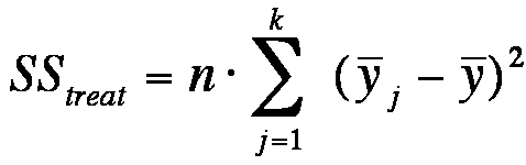
Figure 9: Equation of the treatment variance
whereby
SS = the sum of squared differences
j = the factor level
k = the number of factor levels
n = the sample size
y j = the mean of factor level j
y = the total mean
Differences can also arise through the interaction of the measurement time and the unit of analysis, and they are described as follows:
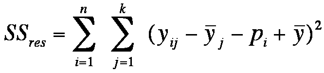
Figure 10: Equation of the residual variance
whereby
SS = the sum of squared differences
j = the factor level
k = the number of factor levels
n = the sample size
yij = the attributes of groups i in factor level j
y j = the mean of factor level j
pi = the mean of all the measured values of group i
y = the total mean
The following table shows the degrees of freedom with which the individual variances are standardized to obtain the respective variances:

Table 2: Degrees of freedom
The F test statistic is derived from the relationship of treatment variance to residual variance:
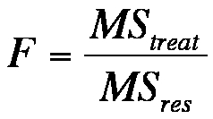
Figure 11: Calculating the test statistic
The F-distributed test statistic is compared with the critical value of the theoretical F-distribution as determined by degrees of freedom.
2.3 Testing for sphericity
Conducting a one-way repeated measures analysis of variance is possible only if the mean differences between the measurement times have homogeneous variances (referred to as “sphericity”). Before conducting the analysis of variance, it is necessary to conduct a sphericity test, which SPSS does automatically.
For the data in this example, SPSS produces a p-value of .001 in the sphericity test (see Chapter 3: “One-way repeated measures analysis of variance with SPSS”). The literature explains that the p-value of the test for sphericity should be greater than .100. The p-value of the example data indicates that sphericity is not given and that the prerequisite of the one-way repeated measures analysis of variance is therefore not met. If the prerequisite of sphericity is violated, SPSS automatically adjusts the degrees of freedom (e.g. based on Greenhouse-Geisser), which then makes it possible to perform further calculations.
2.4 Testing for significance
This section explains how to determine the significance of the calculated test statistic. The F-value is compared with the critical value of the theoretical F-distribution.
For the example data, SPSS shows a test statistic F of 7.664 and a p-value of .001 (see Chapter 3: “One-way repeated measures analysis of variance with SPSS”). In the example data, the prerequisite of sphericity is not met. If the Greenhouse-Geisser epsilon is greater than .750, the Huynh-Feldt p-value needs to be included. In this example, the Greenhouse-Geisser epsilon is smaller than .750. The Greenhouse-Geisser p-value is therefore applied, which is smaller than the significance level of .050. The null hypothesis can be rejected in favor of the alternative hypothesis. The means in the “Desire to Express Worry” scale of husbands differ significantly in at least two measurement times.
Because the analysis of variance with repeated measures tests only if there is at least one difference, it is necessary to afterwards conduct post hoc tests to determine which means differ significantly from the others.
2.5 Post hoc tests
The analysis of variance with repeated measures provides no information about which central tendencies differ significantly from the others.
For this, post hoc tests with paired comparisons of groups can be carried out to determine which differences in the means have caused the analysis of variance with repeated measures to produce a significant result. This involves performing t-tests with paired samples. In the example, six comparisons are made (A&B, A&C, A&D, B&C, B&D, and C&D).
The probability of committing a Type 1 error (the erroneous assumption of an alternative hypothesis) increases with the number of tests carried out. To solve this problem, the significance level is corrected by the number of tests that are carried out. In SPSS, this adjustment can be carried out by selecting “Compare main effects” in the “Repeated measure” menu under “Options” and then choosing “Bonferroni” under “Confidence interval adjustment.”
3. One-way repeated measures analysis of variance with SPSS
This section explains how to define a factor for the repeated measure in SPSS.
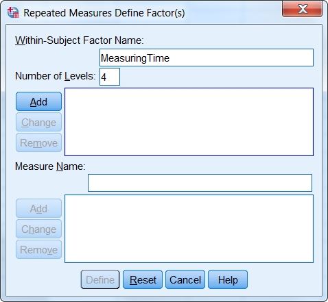
Figure 12: Defining the factor and the “Number of levels.”
In the “Repeated measures” dialogue window, a label can be assigned to a factor under “Within-Subject Factor.” The number of repeated measures is determined under “Number of levels.”
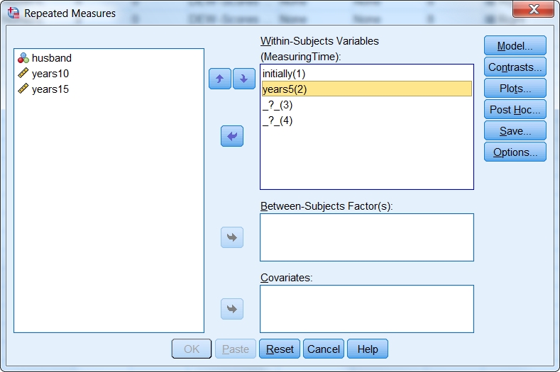
Figure 13: Defining the within-subjects variables
Once the number of factor levels has been determined, a level is assigned chronologically to each measurement time under “Within-subjects variables.”
When carrying out the one-way repeated measures analysis of variance, SPSS produces the following figures, among other things:
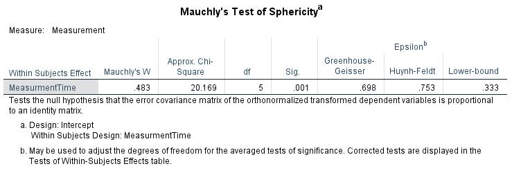
Figure 14: Testing for sphericity
Figure 14 shows Mauchly’s sphericity test. A significant result indicates that sphericity is not given and that the prerequisites of the analysis of variance are not met. SPSS automatically adjusts the degrees of freedom (Greenhouse-Geisser and Huynh-Feldt correction), making further calculations possible.
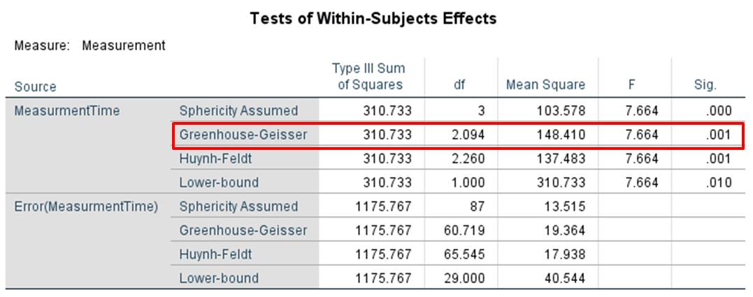
Figure 15: Test statistics and p-values
Figure 15 shows the result of the one-way repeated measures analysis of variance. Because sphericity cannot be assumed in the example data and the Greenhouse-Geisser epsilon is not greater than .750 (see Figure 14), the Greenhouse-Geisser correction becomes relevant (see red marking in Figure 15). In this case, the F-value is 7.664 and the associated p-value is .001. At least one of the differences in the means between the measurement times is significant. However, it is possible to draw specific conclusions about the differences only after the post hoc tests have been conducted.
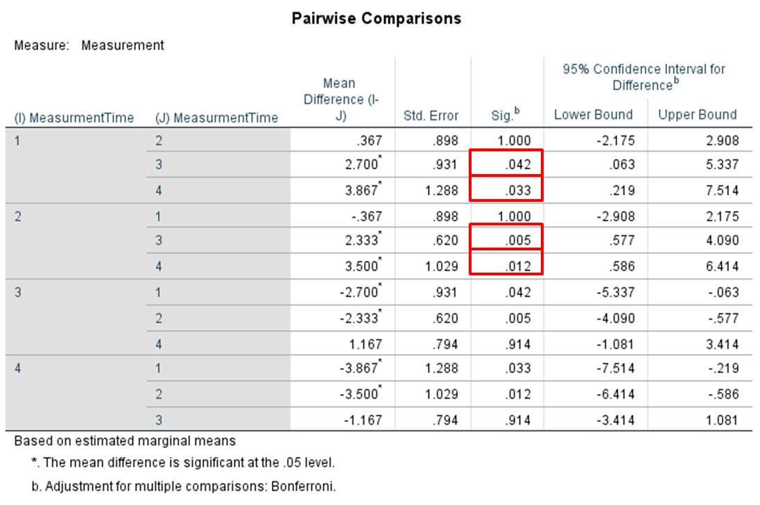
Figure 16: Post hoc tests
In Figure 16, the first column shows the differences in the means between the respective measurement times, whereby the p-values in the third column are relevant. The p-values have been adjusted by means of the Bonferroni correction.
In this example, the mean of husbands on the “Desire to Express Worry” scale right after the wedding differs from the means after 10 and 15 years of marriage. In addition, the mean of the “Desire to Express Worry” scale after 5 years of marriage differs with the means after 10 and 15 years of marriage (see red markings in Figure 16). The differences in the means are significant (the direction of the differences in the means is shown in Figure 3) because the p-values produced by these comparisons are smaller than .050. The probability that husbands will express their worries to their wives declines with the length of the marriage.
4. SPSS commands
SPSS dataset: Example dataset used for the Varianzanalyse-Messwiederholung.sav
Click sequence: Analyze > General linear model > Repeated measures
under “Factor,” define the number of levels (measurement times).
Syntax:
GLM initially years5 years10 years15
/WSFACTOR=Factor1 4 polynomial
/MEASURE = Measurement time
/METHOD=SSTYPE(3)
/PLOT=PROFILE(Factor1)
/EMMEANS = TABLES(Factor1) COMPARE ADJ(BONFERRONI)
/PRINT=DESCRIPTIVE
/CRITERIA=ALPHA(.05)
/WSDESIGN = Factor1.